Glossary
(Internal) Displacement (of humans)
The involuntary movement, individually or collectively, of persons from their country or community, notably for reasons of armed conflict, civil unrest, or natural or human-made disasters (adapted from IOM, 2011).
2030 Agenda for Sustainable Development
A UN resolution in September 2015 adopting a plan of action for people, planet and prosperity in a new global development framework anchored in 17 Sustainable Development Goals (UN, 2015).
Abrupt change
A change in the system that is substantially faster than the typical rate of the changes in its history. See also Abrupt climate change and Tipping point.
Abrupt climate change
A large-scale abrupt change in the climate system that takes place over a few decades or less, persists (or is anticipated to persist) for at least a few decades and causes substantial impacts in human and/or natural systems. See also Tipping point and Abrupt change.
Access to food
See Access under Food security.
Acclimatisation
A change in functional or morphological traits occurring once or repeatedly (e.g., seasonally) during the lifetime of an individual organism in its natural environment. Through acclimatisation, the individual maintains performance across a range of environmental conditions. For a clear differentiation between findings in laboratory and field studies, the term ‘acclimation’ is used in ecophysiology for the respective phenomena when observed in well-defined experimental settings. The term ‘(adaptive) plasticity’ characterises the generally limited scope of changes in phenotype that an individual can reach through the process of acclimatisation.
Accumulation (of glaciers, ice sheets or snow cover)
All processes that add to the mass of a glacier, an ice sheet, or snow cover. The main process of accumulation is snowfall. Accumulation also includes deposition of hoar, freezing rain, other types of solid precipitation, gain of wind-blown snow, avalanching and basal accumulation (often beneath floating ice).
Acute food insecurity
Acute food insecurity is a situation which can occur at any time with a severity that threatens lives, livelihoods or both, regardless of the causes, context or duration, as a result of shocks risking determinants of food security and nutrition, and used to assess the need for humanitarian action (IPC Global Partners, 2019).
Adaptation
In human systems, the process of adjustment to actual or expected climate and its effects, in order to moderate harm or exploit beneficial opportunities. In natural systems, the process of adjustment to actual climate and its effects; human intervention may facilitate adjustment to expected climate and its effects. See also Adaptation options, Adaptive capacity and Maladaptive actions (Maladaptation).
Adaptation deficit
The gap between the current state of a system and a state that minimises adverse impacts from existing climate conditions and variability.
Adaptation gap
The difference between actually implemented adaptation and a societally set goal, determined largely by preferences related to tolerated climate change impacts and reflecting resource limitations and competing priorities (UNEP, 2014; UNEP, 2018).
Adaptation limits
The point at which an actor’s objectives (or system needs) cannot be secured from intolerable risks through adaptive actions.
- Hard adaptation limit – No adaptive actions are possible to avoid intolerable risks.
- Soft adaptation limit – Options may exist but are currently not available to avoid intolerable risks through adaptive action.
Adaptation needs
The circumstances requiring action to ensure the safety of populations and the security of assets in response to climate impacts.
Adaptation options
The array of strategies and measures that are available and appropriate for addressing adaptation. They include a wide range of actions that can be categorised as structural, institutional, ecological or behavioural.
Autonomous adaptation
Adaptation in response to experienced climate and its effects, without planning explicitly or consciously focused on addressing climate change. Also referred to as spontaneous adaptation.
Community-based adaptation
Local, community-driven adaptation. Community-based adaptation focuses attention on empowering and promoting the adaptive capacity of communities. It is an approach that takes context, culture, knowledge, agency and preferences of communities as strengths.
Ecosystem-based adaptation (EBA)
The use of ecosystem management activities to increase the resilience and reduce the vulnerability of people and ecosystems to climate change (Campbell et al., 2009). See also Nature-based solution (NBS).
Evolutionary adaptation
The process whereby a species or population becomes better able to live in a changing environment through the selection of heritable traits. Biologists usually distinguish evolutionary adaptation from acclimatisation, with the latter occurring within an organism’s lifetime.
Incremental adaptation
Adaptation that maintains the essence and integrity of a system or process at a given scale (Park et al., 2012). In some cases, incremental adaptation can accrue to result in transformational adaptation (Tàbara et al., 2018; Termeer et al., 2017). Incremental adaptations to change in climate are understood as extensions of actions and behaviours that already reduce the losses or enhance the benefits of natural variations in extreme weather/climate events.
Transformational adaptation
Adaptation that changes the fundamental attributes of a social-ecological system in anticipation of climate change and its impacts.
Adaptation Fund
A Fund established under the Kyoto Protocol in 2001 and officially launched in 2007. The Fund finances adaptation projects and programmes in developing countries that are Parties to the Kyoto Protocol. Financing comes mainly from sales of Certified Emissions Reductions (CERs) and a share of proceeds amounting to 2% of the value of CERs issued each year for Clean Development Mechanism (CDM) projects. The Adaptation Fund can also receive funds from governments, the private sector and individuals.
Adaptation limits
See Adaptation.
Adaptation needs
See Adaptation.
Adaptation options
See Adaptation.
Adaptation pathways
See Pathways.
Adaptive capacity
The ability of systems, institutions, humans and other organisms to adjust to potential damage, to take advantage of opportunities or to respond to consequences (MA, 2005).
Adaptive governance
See Governance.
Adaptive management
A process of iteratively planning, implementing and modifying strategies for managing resources in the face of uncertainty and change. Adaptive management involves adjusting approaches in response to observations of their effect on, and changes in, the system brought on by resulting feedback effects and other variables.
Adverse side-effect
A negative effect that a policy or measure aimed at one objective has on another objective, thereby potentially reducing the net benefit to society or the environment. See also Trade-off and Co-benefit.
Aerosol
A suspension of airborne solid or liquid particles, with typical particle size in the range of a few nanometres to several tens of micrometres and atmospheric lifetimes of up to several days in the troposphere and up to years in the stratosphere. The term aerosol, which includes both the particles and the suspending gas, is often used in this report in its plural form to mean ‘aerosol particles’. Aerosols may be of either natural or anthropogenic origin in the troposphere; stratospheric aerosols mostly stem from volcanic eruptions. Aerosols can cause an effective radiative forcing directly through scattering and absorbing radiation (aerosol–radiation interaction), and indirectly by acting as cloud condensation nuclei or ice nucleating particles that affect the properties of clouds (aerosol–cloud interaction), and upon deposition on snow- or ice-covered surfaces. Atmospheric aerosols may be either emitted as primary particulate matter or formed within the atmosphere from gaseous precursors (secondary production). Aerosols may be composed of sea salt, organic carbon, black carbon (BC), mineral species (mainly desert dust), sulphate, nitrate and ammonium or their mixtures. See also Particulate matter (PM) and Short-lived climate forcers (SLCFs).
Afforestation
Conversion to forest of land that historically has not contained forests. See also Deforestation.
[Note: For a discussion of the term forest and related terms such as afforestation, reforestation and deforestation, see the 2006 IPCC Guidelines for National Greenhouse Gas Inventories and their 2019 Refinement, and information provided by the United Nations Framework Convention on Climate Change (IPCC 2006, 2019; UNFCCC 2021a, 2021b)]
Agreement
In this report, the degree of agreement within the scientific body of knowledge on a particular finding is assessed based on multiple lines of evidence (e.g., mechanistic understanding, theory, data, models, expert judgement) and expressed qualitatively (Mastrandrea et al., 2010). See also Confidence, Evidence, Likelihood and Uncertainty.
Agricultural and ecological drought
See Drought.
Agroecology
The science and practice of applying ecological concepts, principles and knowledge (i.e., the interactions of, and explanations for, the diversity, abundance and activities of organisms) to the study, design and management of sustainable agroecosystems. It includes the roles of human beings as a central organism in agroecology by way of social and economic processes in farming systems. Agroecology examines the roles and interactions among all relevant biophysical, technical and socioeconomic components of farming systems and their surrounding landscapes (IPBES, 2019).
Agroforestry
Collective name for land-use systems and technologies where woody perennials (trees, shrubs, palms, bamboos, etc.) are deliberately used on the same land-management units as agricultural crops and/or animals, in some form of spatial arrangement or temporal sequence. In agroforestry systems, there are both ecological and economical interactions between the different components. Agroforestry can also be defined as a dynamic, ecologically based, natural resource management system that, through the integration of trees on farms and in the agricultural landscape, diversifies and sustains production for increased social, economic and environmental benefits for land users at all levels (FAO, 2015a).
Air pollution
Degradation of air quality with negative effects on human health or the natural or built environment due to the introduction, by natural processes or human activity, into the atmosphere of substances (gases, aerosols) which have a direct (primary pollutants) or indirect (secondary pollutants) harmful effect.
Albedo
The proportion of sunlight (solar radiation) reflected by a surface or object, often expressed as a percentage. Clouds, snow and ice usually have high albedo; soil surfaces cover the albedo range from high to low; vegetation in the dry season and/or in arid zones can have high albedo, whereas photosynthetically active vegetation and the ocean have low albedo. The Earth’s planetary albedo changes mainly through changes in cloudiness, snow, ice, leaf area and land cover.
Anomaly
The deviation of a variable from its value averaged over a reference period.
Anthropocene
A proposed new geological epoch resulting from significant human-driven changes to the structure and functioning of the Earth system, including the climate system. Originally proposed in the Earth System science community in 2000, the proposed new epoch is undergoing a formalisation process within the geological community based on the stratigraphic evidence that human activities have changed the Earth System to the extent of forming geological deposits with a signature that is distinct from those of the Holocene, and which will remain in the geological record. Both the stratigraphic and Earth system approaches to defining the Anthropocene consider the mid-20th century to be the most appropriate starting date (Steffen et al., 2016), although others have been proposed and continue to be discussed. The Anthropocene concept has already been informally adopted by diverse disciplines and the public to denote the substantive influence of humans on the Earth system.
Anthropogenic
Resulting from or produced by human activities.
Anthropogenic emissions
See Emissions.
Anthropogenic subsidence
Downward motion of the land surface induced by anthropogenic drivers (e.g., loading, extraction of hydrocarbons and/or groundwater, drainage and mining activities) causing sediment compaction or subsidence/deformation of the sedimentary sequence, or oxidation of organic material, thereby leading to relative sea level rise.
Arid zone
Areas where vegetation growth is severely constrained due to limited water availability. For the most part, the native vegetation of arid zones is sparse. There is high rainfall variability, with annual averages below 300 mm. Crop farming in arid zones requires irrigation.
Aridity
The state of a long-term climatic feature characterised by low average precipitation or available water in a region. Aridity generally arises from widespread persistent atmospheric subsidence or anticyclonic conditions, and from more localised subsidence in the lee side of mountains (adapted from Ogallo and Gbeckor-Kove, 1989). See also Drought.
Atmosphere
The gaseous envelope surrounding the Earth, divided into five layers: the troposphere, which contains half of the Earth’s atmosphere, the stratosphere, the mesosphere, the thermosphere and the exosphere, which is the outer limit of the atmosphere. The dry atmosphere consists almost entirely of nitrogen (78.1% volume mixing ratio) and oxygen (20.9% volume mixing ratio), together with a number of trace gases such as argon (0.93% volume mixing ratio), helium and radiatively active greenhouse gases (GHGs) such as carbon dioxide (CO2) (0.04% volume mixing ratio) methane (CH4), nitrous oxide (N2O) and ozone (O3). In addition, the atmosphere contains the GHG water vapour (H2O), whose concentrations are highly variable (0–5% volume mixing ratio) as the sources (evapotranspiration) and sinks (precipitation) of water vapour show large spatio-temporal variations, and atmospheric temperature exerts a strong constraint on the amount of water vapour an air parcel can hold.. The atmosphere also contains clouds and aerosols. See also Hydrological cycle.
Attribution
Attribution is defined as the process of evaluating the relative contributions of multiple causal factors to a change or event with an assessment of confidence.
Autonomous adaptation
See Adaptation.
Avalanche
A mass of snow, ice, earth or rocks, or a mixture of these, falling down a mountainside.
Baseline scenario
see Reference scenario.
Behavioural change
In this report, behavioural change refers to alteration of human decisions and actions in ways that mitigate climate change and/or reduce negative consequences of climate change impacts.
Benthic
Occurring at the bottom of a body of water; related to benthos (NOAA, 2018). See also Benthos.
Benthos
The community of organisms living on the bottom or in sediments of a body of water (such as an ocean, a river or a lake). The ecological zone at the bottom of a body of water, including the sediment surface and some subsurface layers, is known as the benthic zone.
Beta diversity
The change in species composition between different areas (spatial turnover) or times (temporal turnover) due to habitat and environmental heterogeneity
Biodiversity
Biodiversity or biological diversity means the variability among living organisms from all sources including, among other things, terrestrial, marine and other aquatic ecosystems, and the ecological complexes of which they are part; this includes diversity within species, between species and of ecosystems (UN, 1992). See also Ecosystem and Ecosystem services.
Biodiversity hotspots
Biodiversity hotspots are geographic areas exceptionally rich in species, ecologically distinct, and often contain geographically rare endemic species. They are thus priorities for nature conservation action.
Bioenergy
Energy derived from any form of biomass or its metabolic by-products. See also Biofuel and Biomass.
Biofuel
A fuel, generally in liquid form, produced from biomass. Biofuels include bioethanol from sugarcane, sugar beet or maize and biodiesel from canola or soybeans. See also Bioenergy.
Biomass
Organic material excluding the material that is fossilised or embedded in geological formations. Biomass may refer to the mass of organic matter in a specific area (ISO, 2014). See also Bioenergy and Biofuel.
Biomes
Global-scale zones, generally defined by the type of plant life that they support in response to average rainfall and temperature patterns. For example, tundra, coral reefs or savannas (IPBES, 2019).
Biosphere (terrestrial and marine)
The part of the Earth system comprising all ecosystems and living organisms, in the atmosphere, on land (terrestrial biosphere) or in the oceans (marine biosphere), including derived dead organic matter, such as litter, soil organic matter and oceanic detritus.
Blue carbon
Biologically driven carbon fluxes and storage in marine systems that are amenable to management. Coastal blue carbon focuses on rooted vegetation in the coastal zone, such as tidal marshes, mangroves and seagrasses. These ecosystems have high carbon burial rates on a per unit area basis and accumulate carbon in their soils and sediments. They provide many non-climatic benefits and can contribute to ecosystem-based adaptation. If degraded or lost, coastal blue carbon ecosystems are likely to release most of their carbon back to the atmosphere. There is current debate regarding the application of the blue carbon concept to other coastal and non-coastal processes and ecosystems, including the open ocean. See also Ecosystem services and Sequestration.
Blue infrastructure
See Infrastructure.
Burden
The total mass of a gaseous substance of concern in the atmosphere.
Business-As-Usual (BAU)
The term Business-As-Usual scenario has been used to describe a scenario that assumes no additional policies beyond those currently in place and that patterns of socio-economic development are consistent with recent trends. The term is now used less frequently than in the past. See also Reference scenario.
Calcification
The process of biologically precipitating calcium carbonate minerals to create organism shells, skeletons, otoliths or other body structures. The chemical equation describing calcification is Ca2+(aq) + 2HCO3−(aq) → CaCO3(s) + CO2 + H2O. Aragonite and calcite are two common crystalline forms of biologically precipitated calcium carbonate minerals that have different solubilities.
Capacity building
The practice of enhancing the strengths and attributes of, and resources available to, an individual, community, society or organisation to respond to change.
Carbon dioxide (CO2)
A naturally occurring gas, CO2 is also a by-product of burning fossil fuels (such as oil, gas and coal), of burning biomass, of land-use changes (LUC) and of industrial processes (e.g., cement production). It is the principal anthropogenic greenhouse gas (GHG) that affects the Earth’s radiative balance. It is the reference gas against which other GHGs are measured and therefore has a global warming potential (GWP) of 1.
Carbon dioxide (CO2) fertilisation
The increase of plant photosynthesis and water-use efficiency in response to increased atmospheric carbon dioxide (CO2) concentration. Whether this increased photosynthesis translates into increased plant growth and carbon storage on land depends on the interacting effects of temperature, moisture and nutrient availability.
Carbon dioxide removal (CDR)
Anthropogenic activities removing carbon dioxide (CO2) from the atmosphere and durably storing it in geological, terrestrial or ocean reservoirs, or in products. It includes existing and potential anthropogenic enhancement of biological or geochemical CO2 sinks and direct air carbon dioxide capture and storage (DACCS) but excludes natural CO2 uptake not directly caused by human activities. See also Afforestation.
Carbon footprint
Measure of the exclusive total amount of emissions of carbon dioxide (CO2) that is directly and indirectly caused by an activity or accumulated over the life stages of a product (Wiedmann and Minx, 2008).
Carbon stock
The quantity of carbon in a carbon pool.
Cascading impacts
Cascading impacts from extreme weather/climate events occur when an extreme hazard generates a sequence of secondary events in natural and human systems that result in physical, natural, social or economic disruption, whereby the resulting impact is significantly larger than the initial impact. Cascading impacts are complex and multi-dimensional, and are associated more with the magnitude of vulnerability than with that of the hazard (modified from Pescaroli & Alexander, 2015).
Catchment
An area that collects and drains precipitation.
Cities
Cities are open systems, continually exchanging resources, products and services, waste, people, ideas and finances with the hinterlands and broader world. Cities are complex, self-organising, adaptive and constantly evolving. Cities also encompass multiple actors with varying responsibilities, capabilities and priorities, as well as processes that transcend the institutional sector-based approach to city administration. Cities are embedded in broader ecological, economic, technical, institutional, legal and governance structures that enable or constrain their systemic function, which cannot be separated from wider power relations. Urban processes of a physical, social and economic nature are causally interlinked, with interactions and feedbacks that result in both intended and unintended impacts on emissions. See also City region, Peri-urban areas and Urban.
City region
The areal extent of an individual city’s material associations and economic or political influence. The city region concept accepts that rural livelihoods and land uses can be incorporated within the functional activities of a city. This will include dormitory settlements, sources for critical inputs of water, some food, and waste disposal. See also Region, Cities, Urban and Urban systems.
Climate
In a narrow sense, climate is usually defined as the average weather -or more rigorously, as the statistical description in terms of the mean and variability of relevant quantities- over a period of time ranging from months to thousands or millions of years. The classical period for averaging these variables is 30 years, as defined by the World Meteorological Organization (WMO). The relevant quantities are most often surface variables such as temperature, precipitation and wind. Climate in a wider sense is the state, including a statistical description, of the climate system.
Climate change
A change in the state of the climate that can be identified (e.g., by using statistical tests) by changes in the mean and/or the variability of its properties and that persists for an extended period, typically decades or longer. Climate change may be due to natural internal processes or external forcings such as modulations of the solar cycles, volcanic eruptions and persistent anthropogenic changes in the composition of the atmosphere or in land use. Note that the United Nations Framework Convention on Climate Change (UNFCCC), in its Article 1, defines climate change as: ‘a change of climate which is attributed directly or indirectly to human activity that alters the composition of the global atmosphere and which is in addition to natural climate variability observed over comparable time periods’. The UNFCCC thus makes a distinction between climate change attributable to human activities altering the atmospheric composition and climate variability attributable to natural causes. See also Climate variability, Detection, Attribution and Ocean acidification (OA).
Climate extreme (extreme weather or climate event)
The occurrence of a value of a weather or climate variable above (or below) a threshold value near the upper (or lower) ends of the range of observed values of the variable.
By definition, the characteristics of what is called extreme weather may vary from place to place in an absolute sense. When a pattern of extreme weather persists for some time, such as a season, it may be classified as an extreme climate event, especially if it yields an average or total that is itself extreme (e.g., high temperature, drought or heavy rainfall over a season). For simplicity, both extreme weather events and extreme climate events are referred to collectively as climate extremes.
Climate feedback
An interaction in which a perturbation in one climate quantity causes a change in a second and the change in the second quantity ultimately leads to an additional change in the first. A negative feedback is one in which the initial perturbation is weakened by the changes it causes; a positive feedback is one in which the initial perturbation is enhanced. The initial perturbation can either be externally forced or arise as part of internal variability.
Climate finance
There is no agreed definition of climate finance. The term climate finance is applied to the financial resources devoted to addressing climate change by all public and private actors from global to local scales, including international financial flows to developing countries to assist them in addressing climate change. Climate finance aims to reduce net greenhouse gas emissions and/or to enhance adaptation and increase resilience to the impacts of current and projected climate change. Finance can come from private and public sources, channelled by various intermediaries, and is delivered by a range of instruments, including grants, concessional and non-concessional debt, and internal budget reallocations.
Climate governance
See Governance.
Climate information
Information about the past, current or future state of the climate system that is relevant for mitigation, adaptation and risk management. It may be tailored or “co-produced” for specific contexts, taking into account users’ needs and values.
Climate justice
See Justice.
Climate literacy
Climate literacy encompasses being aware of climate change, its anthropogenic causes and implications.
Climate model
A qualitative or quantitative representation of the climate system based on the physical, chemical and biological properties of its components, their interactions and feedback processes and accounting for some of its known properties. The climate system can be represented by models of varying complexity; that is, for any one component or combination of components, a spectrum or hierarchy of models can be identified, differing in such aspects as the number of spatial dimensions, the extent to which physical, chemical or biological processes are explicitly represented, or the level at which empirical parametrisations are involved. There is an evolution towards more complex models with interactive chemistry and biology. Climate models are applied as a research tool to study and simulate the climate and for operational purposes, including monthly, seasonal and interannual climate predictions. See also Earth system model (ESM).
Climate prediction
A climate prediction or climate forecast is the result of an attempt to produce (starting from a particular state of the climate system) an estimate of the actual evolution of the climate in the future, for example, at seasonal, interannual or decadal time scales. Because the future evolution of the climate system may be highly sensitive to initial conditions, such predictions are usually probabilistic in nature.
Climate projection
Simulated response of the climate system to a scenario of future emissions or concentrations of greenhouse gases (GHGs) and aerosols and changes in land use, generally derived using climate models. Climate projections depend on an emission/concentration/radiative forcing scenario, which is in turn based on assumptions concerning, for example, future socioeconomic and technological developments that may or may not be realised.
Climate refugium
A climate refugium is a geographic area that has had a stable climate on evolutionary time scales, or that is projected to have a stable climate into the future. See also Refugium.
Climate services
Climate services involve the provision of climate information in such a way as to assist decision-making. The service includes appropriate engagement from users and providers, is based on scientifically credible information and expertise, has an effective access mechanism and responds to user needs (Hewitt et al. 2012).
Climate simulation ensemble
A group of parallel model simulations characterising historical climate conditions, climate predictions or climate projections. Variation of the results across the ensemble members may give an estimate of modelling-based uncertainty. Ensembles made with the same model but different initial conditions characterise the uncertainty associated with internal climate variability, whereas multi-model ensembles including simulations by several models also include the effect of model differences. Perturbed parameter ensembles, in which model parameters are varied in a systematic manner, aim to assess the uncertainty resulting from internal model specifications within a single model. Remaining sources of uncertainty unaddressed with model ensembles are related to systematic model errors or biases, which may be assessed from systematic comparisons of model simulations with observations wherever available.
Climate system
The global system consisting of five major components: the atmosphere, the hydrosphere, the cryosphere, the lithosphere and the biosphere and the interactions between them. The climate system changes in time under the influence of its own internal dynamics and because of external forcings such as volcanic eruptions, solar variations, orbital forcing, and anthropogenic forcings such as the changing composition of the atmosphere and land-use change.
Climate variability
Deviations of some climate variables from a given mean state (including the occurrence of extremes, etc.) at all spatial and temporal scales beyond that of individual weather events. Variability may be intrinsic, due to fluctuations of processes internal to the climate system (internal variability), or extrinsic, due to variations in natural or anthropogenic external forcing (forced variability).
Climate velocity
The speed at which isolines of a specified climate variable travel across landscapes or seascapes due to changing climate. For example, climate velocity for temperature is the speed at which isotherms move due to changing climate (km yr−1) and is calculated as the temporal change in temperature (°C yr−1) divided by the current spatial gradient in temperature (°C km−1). It can be calculated using additional climate variables such as precipitation or can be based on the climatic niche of organisms.
Climate resilient development
In the WGII report, climate resilient development refers to the process of implementing greenhouse gas mitigation and adaptation measures to support sustainable development for all.
Climate resilient development pathways (CRDPs)
See Pathways.
Climate-resilient pathways
See Pathways.
Climate-smart agriculture (CSA)
An approach to agriculture that aims to transform and reorient agricultural systems to effectively support development and ensure food security in a changing climate by sustainably increasing agricultural productivity and incomes, adapting and building resilience to climate change, and reducing and/or removing greenhouse gas emissions, where possible (FAO, 2018).
Climatic driver (Climate driver)
A changing aspect of the climate system that influences a component of a human or natural system.
Climatic impact-drivers (CIDs)
Climatic impact-drivers (CIDs) are physical climate system conditions (e.g., means, events, extremes) that affect an element of society or ecosystems. Depending on system tolerance, CIDs and their changes can be detrimental, beneficial, neutral, or a mixture of each across interacting system elements and regions.
CMIP3, CMIP5 and CMIP6
See Coupled Model Intercomparison Project (CMIP).
Co-benefit
A positive effect that a policy or measure aimed at one objective has on another objective, thereby increasing the total benefit to society or the environment. Co-benefits are also referred to as ancillary benefits. See also Trade-off and Adverse side-effect.
Coast
The land near to the sea. The term ‘coastal’ can refer to that land (e.g., as in ‘coastal communities’), or to that part of the marine environment that is strongly influenced by land-based processes. Thus, coastal seas are generally shallow and near-shore. The landward and seaward limits of the coastal zone are not consistently defined, neither scientifically nor legally. Thus, coastal waters can either be considered as equivalent to territorial waters (extending 12 nautical miles/22.2 km from mean low water), or to the full exclusive economic zone, or to shelf seas, with less than 200 m water depth.
Coastal erosion
Coastal erosion, sometimes referred to as shoreline retreat, occurs when a net loss of sediment or bedrock from the shoreline results in landward movement of the high-tide mark.
Communicable disease
Illness due to a specific infectious agent or its toxic products that arises through transmission of that agent or its products from an infected person, animal or reservoir to a susceptible host, either directly or indirectly through an intermediate plant or animal host, vector or the inanimate environment. Communicable disease pathogens include bacteria, viruses, fungi, parasites and prions.
Community-based adaptation
See Adaptation.
Compound risks
See Risk.
Compound weather/climate events
The terms ‘compound events’, ‘compound extremes’ and ‘compound extreme events’ are used interchangeably in the literature and this report and refer to the combination of multiple drivers and/or hazards that contributes to societal and/or environmental risk (Zscheischler et al., 2018).
Concentrations scenario
See Scenarios.
Confidence
The robustness of a finding based on the type, amount, quality and consistency of evidence (e.g., mechanistic understanding, theory, data, models, expert judgment) and on the degree of agreement across multiple lines of evidence. In this report, confidence is expressed qualitatively (Mastrandrea et al., 2010).
Conservation agriculture
A farming system that promotes minimum soil disturbance (e.g., by using no-till practices), maintenance of a permanent soil cover and diversification of plant species. It aims to prevent land degradation and regenerate degraded lands by enhancing biodiversity and natural biological processes above and below the ground surface that contribute to increased water and nutrient use efficiency and improved and sustained crop production (FAO, 2016).
Coping
The use of available skills, resources and opportunities to address, manage and overcome adverse conditions, with the aim of achieving basic functioning of people, institutions, organisations and systems in the short to medium term (UNISDR, 2009; IPCC, 2012a).
Coping capacity
The ability of people, institutions, organisations and systems, using available skills, values, beliefs, resources and opportunities, to address, manage and overcome adverse conditions in the short to medium term (UNISDR, 2009; IPCC, 2012a). See also Resilience.
Coral bleaching
Loss of coral pigmentation through the loss of intracellular symbiotic algae (known as zooxanthellae) and/or loss of their pigments.
Coral reef
An underwater ecosystem characterised by structure-building stony corals. Warm-water coral reefs occur in shallow seas, mostly in the tropics, with the corals (animals) containing algae (plants) that depend on light and relatively stable temperature conditions. Cold-water coral reefs occur throughout the world, mostly at water depths of 50–500 m. In both kinds of reef, living corals frequently grow on older, dead material, predominantly made of calcium carbonate (CaCO3). Both warm- and cold-water coral reefs support high biodiversity of fish and other groups, and are considered to be especially vulnerable to climate change.
Cost–benefit analysis
Monetary assessment of all negative and positive impacts associated with a given action. Cost–benefit analysis enables comparison of different interventions, investments or strategies and reveals how a given investment or policy effort pays off for a particular person, company or country. Cost–benefit analyses representing society’s point of view are important for climate change decision-making, but there are difficulties in aggregating costs and benefits across different actors and across timescales. See also Discounting.
Coupled Model Intercomparison Project (CMIP)
A climate modelling activity from the World Climate Research Programme (WCRP) which coordinates and archives climate model simulations based on shared model inputs by modelling groups from around the world. The CMIP3 multi-model data set includes projections using Special Report on Emissions Scenarios (SRES) scenarios. The CMIP5 data set includes projections using the Representative Concentration Pathways (RCP). The CMIP6 phase involves a suite of common model experiments as well as an ensemble of CMIP-endorsed Model Intercomparison Projects (MIPs).
Cryosphere
The components of the Earth system at and below the land and ocean surface that are frozen, including snow cover, glaciers, ice sheets, ice shelves, icebergs, sea ice, lake ice, river ice, permafrost and seasonally frozen ground.
Cultural impacts
Impacts on material and ecological aspects of culture and the lived experience of culture, including dimensions such as identity, community cohesion and belonging, sense of place, worldview, values, perceptions and tradition. Cultural impacts are closely related to ecological impacts, especially for iconic and representational dimensions of species and landscapes. Culture and cultural practices frame the importance and value of the impacts of change, shape the feasibility and acceptability of adaptation options, and provide the skills and practices that enable adaptation.
Decarbonisation
Human actions to reduce carbon dioxide emissions from human activities.
Deep uncertainty
See Uncertainty.
Deforestation
Conversion of forest to non-forest. See also Afforestation and Reforestation.
[Note: For a discussion of the term forest and related terms such as afforestation, reforestation and deforestation, see the 2006 IPCC Guidelines for National Greenhouse Gas Inventories and their 2019 Refinement, and information provided by the United Nations Framework Convention on Climate Change (IPCC 2006, 2019; UNFCCC 2021a, 2021b)]
Desertification
Land degradation in arid, semi-arid, and dry sub-humid areas resulting from many factors, including climatic variations and human activities (UNCCD, 1994).
Detection
Detection of change is defined as the process of demonstrating that climate or a system affected by climate has changed in some defined statistical sense, without providing a reason for that change. An identified change is detected in observations if its likelihood of occurrence by chance due to internal variability alone is determined to be small, for example, <10%.
Detection and attribution
See Attribution and Detection.
Developed/developing countries (Industrialised/developed/developing countries)
There is a diversity of approaches for categorising countries on the basis of their level of development, and for defining terms such as ‘industrialised’, ‘developed’ or ‘developing’. Several categorisations are used in this Special Report. (1) In the United Nations (UN) system, there is no established convention for the designation of developed and developing countries or areas. (2) The UN Statistics Division specifies developed and developing regions based on common practice. In addition, specific countries are designated as Least Developed Countries, landlocked developing countries, Small Island Developing States (SIDS) and transition economies. Many countries appear in more than one of these categories. (3) The World Bank uses income as the main criterion for classifying countries as low, lower middle, upper middle and high income. (4) The UN Development Programme (UNDP) aggregates indicators for life expectancy, educational attainment and income into a single composite Human Development Index (HDI) to classify countries as low, medium, high or very high human development.
Development pathways
See Pathways.
Diatoms
Microscopic (2–200 µm) unicellular photosynthetic algae that live in surface waters of lakes, rivers and oceans and form shells of opal. In the global ocean, marine diatom species distribution is primarily driven by nutrient availability. On regional scales, their species distribution in ocean sediment cores can be related to past sea surface temperatures.
Diet
The kinds of food that follow a particular pattern that a person or community eats (FAO, 2014).
Disaster
A ‘serious disruption of the functioning of a community or a society at any scale due to hazardous events interacting with conditions of exposure, vulnerability and capacity, leading to one or more of the following: human, material, economic and environmental losses and impacts’ (UNGA, 2016). See also Exposure, Hazard, Risk and Vulnerability.
Disaster management
Social processes for designing, implementing and evaluating strategies, policies and measures that promote and improve disaster preparedness, response and recovery practices at different organisational and societal levels.
Disaster risk
The likelihood over a specified time period of severe alterations in the normal functioning of a community or a society due to hazardous physical events interacting with vulnerable social conditions, leading to widespread adverse human, material, economic or environmental effects that require immediate emergency response to satisfy critical human needs and that may require external support for recovery.
Disaster risk management (DRM)
Processes for designing, implementing and evaluating strategies, policies and measures to improve the understanding of current and future disaster risk, foster disaster risk reduction and transfer, and promote continuous improvement in disaster preparedness, prevention and protection, response and recovery practices, with the explicit purpose of increasing human security, well-being, quality of life and sustainable development (SD).
Disaster risk reduction (DRR)
Denotes both a policy goal or objective, and the strategic and instrumental measures employed for anticipating future disaster risk; reducing existing exposure, hazard or vulnerability; and improving resilience.
Discount rate
See Discounting.
Discounting
A mathematical operation that aims to make monetary (or other) amounts received or expended at different times (years) comparable across time. If the discount rate is positive, future values are given less weight than those today. The choice of discount rate(s) is debated as it is a judgement based on hidden and/or explicit values.
Downscaling
A method that derives local- to regional-scale information from larger-scale models or data analyses. Two main methods exist: dynamical downscaling and empirical/statistical downscaling. The dynamical method uses the output of regional climate models, global models with variable spatial resolution or high-resolution global models. The empirical/statistical methods are based on observations and develop statistical relationships that link the large-scale atmospheric variables with local/regional climate variables. In all cases, the quality of the driving model remains an important limitation on the quality of the downscaled information. The two methods can be combined, for example, applying empirical/statistical downscaling to the output of a regional climate model, consisting of a dynamical downscaling of a global climate model.
Drainage
Artificial lowering of the soil water table (IPCC, 2013).
Driver
Any natural or human-induced factor that directly or indirectly causes a change in a system (adapted from MA, 2005). See also Climatic driver.
Drought
An exceptional period of water shortage for existing ecosystems and the human population (due to low rainfall, high temperature and/or wind).
Megadrought
A very lengthy and pervasive drought, lasting much longer than normal, usually a decade or more.
Hydrological drought
A period with large runoff and water deficits in rivers, lakes and reservoirs.
Agricultural and ecological drought
Agricultural and ecological drought (depending on the affected biome): a period with abnormal soil moisture deficit, which results from combined shortage of precipitation and excess evapotranspiration, and during the growing season impinges on crop production or ecosystem function in general.
Meteorological drought
A period with an abnormal precipitation deficit.
Early warning systems (EWS)
The set of technical and institutional capacities to forecast, predict and communicate timely and meaningful warning information to enable individuals, communities, managed ecosystems and organisations threatened by a hazard to prepare to act promptly and appropriately to reduce the possibility of harm or loss. Dependent upon context, EWS may draw upon scientific and/or indigenous knowledge, and other knowledge types. EWS are also considered for ecological applications, for example, conservation, where the organisation itself is not threatened by hazard but the ecosystem under conservation is (e.g., coral bleaching alerts), in agriculture (e.g., warnings of heavy rainfall, drought, ground frost and hailstorms) and in fisheries (e.g., warnings of storms, storm surges and tsunamis) (UNISDR 2009; IPCC, 2012a).
Earth system model (ESM)
A coupled Atmosphere–Ocean General Circulation Model (AOGCM) in which a representation of the carbon cycle is included, allowing for interactive calculation of atmospheric carbon dioxide (CO2) or compatible emissions. Additional components (e.g., atmospheric chemistry, ice sheets, dynamic vegetation, nitrogen cycle, but also urban or crop models) may be included.
Eastern boundary upwelling system (EBUS)
Eastern boundary upwelling systems (EBUS) are located at the eastern (landward) edges of major ocean basins in both hemispheres, where equatorward winds drive upwelling currents that bring cool, nutrient-rich (and often oxygen-poor) waters from the deep ocean to the surface near the coast.
Ecosystem
A functional unit consisting of living organisms, their non-living environment and the interactions within and between them. The components included in a given ecosystem and its spatial boundaries depend on the purpose for which the ecosystem is defined: in some cases, they are relatively sharp, while in others they are diffuse. Ecosystem boundaries can change over time. Ecosystems are nested within other ecosystems, and their scale can range from very small to the entire biosphere. In the current era, most ecosystems either contain people as key organisms or are influenced by the effects of human activities in their environment. See also Ecosystem services and Ecosystem health.
Ecosystem health
Ecosystem health is a metaphor used to describe the condition of an ecosystem, by analogy with human health. Note that there is no universally accepted benchmark for a healthy ecosystem. Rather, the apparent health status of an ecosystem is judged on the ecosystem’s resilience to change, with details depending upon which metrics are employed in judging it and which societal aspirations are driving the assessment (following IPBES 2019).
Ecosystem services
Ecological processes or functions having monetary or non-monetary value to individuals or society at large. These are frequently classified as (1) supporting services such as productivity or biodiversity maintenance, (2) provisioning services such as food or fibre, (3) regulating services such as climate regulation or carbon sequestration and (4) cultural services such as tourism or spiritual and aesthetic appreciation. See also Ecosystem and Ecosystem health.
Ecosystem-based adaptation (EBA)
See Adaptation.
El Niño-Southern Oscillation (ENSO)
The term ‘El Niño’ was initially used to describe a warm-water current that periodically flows along the coast of Ecuador and Peru, disrupting the local fishery. It has since become identified with warming of the tropical Pacific Ocean east of the dateline. This oceanic event is associated with a fluctuation of a global-scale tropical and subtropical surface pressure pattern called the Southern Oscillation. This coupled atmosphere–ocean phenomenon, with preferred time scales of 2 to about 7 years, is known as the El Niño-Southern Oscillation (ENSO). The warm and cold phases of the ENSO are called El Niño and La Niña, respectively. ENSO is often measured by the surface pressure anomaly difference between Tahiti and Darwin and/or the sea surface temperatures in the central and eastern equatorial Pacific. This phenomenon has a great impact on the wind, sea surface temperature and precipitation patterns in the tropical Pacific. It has climatic effects throughout the Pacific region and in many other parts of the world through global teleconnections. See WGI AR6 Annex AIV.2.3 (IPCC 2021a).
Emergence (of the climate signal)
Emergence of a climate change signal or trend refers to when a change in climate (the ‘signal’) becomes larger than the amplitude of natural or internal variations (defining the ‘noise’), This concept is often expressed as a signal-to-noise ratio, and emergence occurs at a defined threshold of this ratio (e.g., S/N > 1 or 2). Emergence can refer to changes relative to a historical or modern baseline (usually at least 20 years long) and can also be expressed in terms of time (time of emergence) or in terms of a global warming level. Emergence is also used to refer to a time when we can expect to see a response of reducing greenhouse gas (GHG) emissions (emergence with respect to mitigation). Emergence can be estimated using observations and/or model simulations.
Emission pathways
See Pathways.
Emission scenario
See Scenario.
Emissions
Anthropogenic emissions
Emissions of greenhouse gases (GHGs), precursors of GHGs and aerosols caused by human activities. These activities include the burning of fossil fuels, deforestation, land use and land-use changes (LULUC), livestock production, fertilisation, waste management and industrial processes.
Fossil-fuel emissions
Emissions of greenhouse gases (in particular, carbon dioxide), other trace gases and aerosols resulting from the combustion of fuels from fossil carbon deposits such as oil, gas and coal.
Non-CO2 emissions and radiative forcing
Non-CO2 emissions included in this report are all anthropogenic emissions other than CO2 that result in radiative forcing. These include short-lived climate forcers, such as methane (CH4), some fluorinated gases, ozone (O3) precursors, aerosols or aerosol precursors, such as black carbon and sulphur dioxide, respectively, as well as long-lived greenhouse gases, such as nitrous oxide (N2O) or other fluorinated gases. The radiative forcing associated with non-CO2 emissions and changes in surface albedo is referred to as non-CO2 radiative forcing.
Enabling conditions (for adaptation and mitigation options)
Conditions that enhance the feasibility of adaptation and mitigation options. Enabling conditions include finance, technological innovation, strengthening policy instruments, institutional capacity, multi-level governance and changes in human behaviour and lifestyles.
Endemic species
Plants and animals that are only found in one geographic region.
Energy access
Access to clean, reliable and affordable energy services for cooking and heating, lighting, communications and productive uses (with special reference to Sustainable Development Goal 7) (AGECC, 2010).
Energy efficiency
The ratio of output or useful energy or energy services or other useful physical outputs obtained from a system, conversion process, transmission or storage activity to the input of energy (measured as kWh kWh−1, tonnes kWh−1 or any other physical measure of useful output like tonne-km transported). Energy efficiency is often described by energy intensity.
Energy security
The goal of a given country, or the global community as a whole, to maintain an adequate, stable and predictable energy supply. Measures encompass safeguarding the sufficiency of energy resources to meet national energy demand at competitive and stable prices and the resilience of the energy supply; enabling the development and deployment of technologies; building sufficient infrastructure to generate, store and transmit energy supplies and ensuring enforceable contracts of delivery.
Energy system
The energy system comprises all components related to the production, conversion, delivery and use of energy.
Equality
A principle that ascribes equal worth to all human beings, including equal opportunities, rights and obligations, irrespective of origins. See also Equity and Fairness.
Inequality
Uneven opportunities and social positions, and processes of discrimination within a group or society, based on gender, class, ethnicity, age and (dis)ability, often produced by uneven development. Income inequality refers to gaps between the highest and lowest income earners within a country and between countries.
Equity
The principle of being fair and impartial, and a basis for understanding how the impacts and responses to climate change, including costs and benefits, are distributed in and by society in more or less equal ways. Often aligned with ideas of equality, fairness and justice and applied with respect to equity in the responsibility for, and distribution of, climate impacts and policies across society, generations and gender, and in the sense of who participates and controls the processes of decision-making.
Ethics
Ethics involves questions of justice and value. Justice is concerned with right and wrong, equity and fairness, and, in general, with the rights to which people and living beings are entitled. Value is a matter of worth, benefit or good.
Eutrophication
Over-enrichment of water by nutrients such as nitrogen and phosphorus. It is one of the leading causes of water quality impairment. The two most acute symptoms of eutrophication are hypoxia (or oxygen depletion) and harmful algal blooms.
Evaporation
The physical process by which a liquid (e.g., water) becomes a gas (e.g., water vapour).
Evapotranspiration
The combined processes through which water is transferred to the atmosphere from open water and ice surfaces, bare soil and vegetation that make up the Earth’s surface.
Evidence
Data and information used in the scientific process to establish findings. In this report, the degree of evidence reflects the amount, quality and consistency of scientific/technical information on which the Lead Authors are basing their findings. See also Agreement, Confidence, Likelihood and Uncertainty.
Evolutionary adaptation
See Adaptation.
Exposure
The presence of people; livelihoods; species or ecosystems; environmental functions, services, and resources; infrastructure; or economic, social, or cultural assets in places and settings that could be adversely affected.
Externality/external cost/external benefit
Externalities arise from a human activity, when agents responsible for the activity do not take full account of the activity’s impact on others’ production and consumption possibilities, and no compensation exists for such impacts. When the impact is negative, they are external costs. When positive they are referred to as external benefits. See also Co-benefits.
Extinction
A population, species or more inclusive taxonomic group has gone extinct when all its individuals have died. A species may go extinct locally (population extinction), regionally (e.g., extinction of all populations in a country, continent or ocean) or globally (IPBES, 2019). See also Extirpation.
Extirpation
The disappearance of a species from an area, sometimes also referred to as local extinction. Its use implies that the species still occurs elsewhere. See also Extinction.
Extreme sea level (ESL)
The occurrence of an exceptionally low or high local sea surface height, arising from (a combination of) short-term phenomena (e.g., storm surges, tides and waves). Relative sea level changes affect extreme sea levels directly by shifting the mean water levels and indirectly by modulating the propagation of tides, waves and/or surges due to increased water depth. In addition, extreme sea levels can be influenced by changes in the frequency, tracks or strength of weather systems and storms, or due to anthropogenically induced changes such as the modification of coastlines or dredging. In turn, changes in any or all of the contributions to extreme sea levels may lead to long-term relative sea level changes. Alternate expressions for ESL may be used depending on the processes resolved.
Extreme still water level (ESWL) refers to the combined contribution of relative sea level change, tides and storm surges. Wind-waves also contribute to coastal sea level via three processes: infragravity waves (lower-frequency gravity waves generated by wind waves), wave setup (time-mean sea level elevation due to wave energy dissipation) and swash (vertical displacement up the shore-face induced by individual waves). Extreme total water level (ETWL) is the ESWL plus wave setup. When considering coastal impacts, swash is also important, and extreme coastal water level (ECWL) is used. See also Sea level change (sea level rise/sea level fall)
Extreme weather event
An event that is rare at a particular place and time of year. Definitions of ‘rare’ vary, but an extreme weather event would normally be as rare as or rarer than the 10th or 90th percentile of a probability density function estimated from observations. By definition, the characteristics of what is called extreme weather may vary from place to place in an absolute sense. See also Heatwave and Climate extreme.
Extreme/heavy precipitation event
An extreme/heavy precipitation event is an event that is of very high magnitude with a very rare occurrence at a particular place. Types of extreme precipitation may vary depending on its duration, hourly, daily or multi-days (e.g., 5 days), though all of them qualitatively represent high magnitude. The intensity of such events may be defined with block maxima approach such as annual maxima or with peak over threshold approach, such as rainfall above 95th or 99th percentile at a particular space.
Fairness
Impartial and just treatment without favouritism or discrimination in which each person is considered of equal worth with equal opportunity. See also Equality and Equity.
Feasibility
In this report, feasibility refers to the potential for a mitigation or adaptation option to be implemented. Factors influencing feasibility are context dependent, temporally dynamic and may vary between different groups and actors. Feasibility depends on geophysical, environmental-ecological, technological, economic, socio-cultural and institutional factors that enable or constrain the implementation of an option. The feasibility of options may change when different options are combined, and increase when enabling conditions are strengthened. See also Enabling conditions (for adaptation and mitigation options).
Fire weather
Weather conditions conducive to triggering and sustaining wildfires, usually based on a set of indicators and combinations of indicators including temperature, soil moisture, humidity and wind. Fire weather does not include the presence or absence of fuel load.
Flood
The overflowing of the normal confines of a stream or other water body, or the accumulation of water over areas that are not normally submerged. Floods can be caused by unusually heavy rain, for example during storms and cyclones. Floods include river (fluvial) floods, flash floods, urban floods, rain (pluvial) floods, sewer floods, coastal floods, and glacial lake outburst floods (GLOF).
Flux
A movement (flow) of matter (e.g., water vapour, particles), heat or energy from one place to another, or from one medium (e.g., land surface) to another (e.g., atmosphere).
Food security
A situation that exists when all people, at all times, have physical, social and economic access to sufficient, safe and nutritious food that meets their dietary needs and food preferences for an active and healthy life. The four pillars of food security are availability, access, utilisation and stability. The nutritional dimension is integral to the concept of food security (FAO, 2018/ 2009).
Availability
Physical availability of food. Food availability addresses the supply side of food security and is determined by the levels of food production, stocks and net trade.
Access
Economic and/or physical access to food. Economic access is determined by disposable income, food prices and the provision of and access to social support. Physical access is determined by the availability and quality of land and other infrastructure, property rights or the functioning of markets.
Utilisation
The way in which the body uses the various nutrients in food. Individuals achieve sufficient energy and nutrient intake through good care and feeding practices, food preparation, diet diversity and intrahousehold distribution of food. Combined with biological utilisation of the food consumed, energy and nutrient intake determine the nutrition status of individuals.
Stability
The stability of the other three dimensions over time. Even if individuals’ food intake is adequate today, they are still considered food-insecure if periodically they have inadequate access to food, risking deterioration of their nutrition status. Adverse weather conditions, political instability or economic factors (unemployment, rising food prices) may have an impact on individuals’ food security status.
Food system
All the elements (environment, people, inputs, processes, infrastructures, institutions, etc.) and activities that relate to the production, processing, distribution, preparation and consumption of food, and the output of these activities, including socio-economic and environmental outcomes (HLPE, 2017). [Note: While there is a global food system (encompassing the totality of global production and consumption), each location’s food system is unique, being defined by that place’s mix of food produced locally, nationally, regionally or globally.]
Food-borne diseases
Illnesses transmitted through the consumption of unsafe or contaminated food. That contamination can come from a variety of sources, including contaminated water (adapted from UNEP, 2018).
Forest
A vegetation type dominated by trees. Many definitions of the term forest are in use throughout the world, reflecting wide differences in bio-geophysical conditions, social structure and economics. See also Afforestation, Deforestation and Reforestation
[Note: For a discussion of the term forest in the context of national GHG inventories, see the 2006 IPCC Guidelines for National GHG Inventories and their 2019 Refinement, and information provided by the United Nations Framework Convention on Climate Change (IPCC 2006, 2019; UNFCCC, 2021a, 2021b).]
Forest degradation
A reduction in the capacity of a forest to produce ecosystem services such as carbon storage and wood products as a result of anthropogenic and environmental changes.
Forest dieback
See Forest degradation.
Forest line
The upper limit of the closed upper montane forest or forest at high latitudes. It is less elevated or less poleward than the tree line.
Forest management
See Sustainable forest management.
Fossil fuels
Carbon-based fuels from fossil hydrocarbon deposits, including coal, oil and natural gas.
Glacial lake outburst flood (GLOF)/Glacier lake outburst
A sudden release of water from a glacier lake, including any of the following types: a glacier-dammed lake, a pro-glacial moraine-dammed lake or water that was stored within, under or on the glacier.
Glacier
A perennial mass of ice, and possibly firn and snow, originating on the land surface by accumulation and compaction of snow and showing evidence of past or present flow. A glacier typically gains mass by accumulation of snow and loses mass by ablation. Land ice masses of continental size (>50,000 km2) are referred to as ice sheets (Cogley et al., 2011).
Global change
A generic term to describe global-scale changes in systems, including the climate system, ecosystems and social-ecological systems.
Global mean sea level change
Global mean sea level (GMSL) change is the increase or decrease in the volume of the ocean divided by the ocean surface area. It is the sum of changes in ocean density through temperature changes (global mean thermosteric sea level change) and changes in the ocean mass as a result of changes in the cryosphere or land water storage (barystatic sea level change).
Global mean surface air temperature (GSAT)
The global average of near-surface air temperatures over land, oceans and sea ice. Changes in GSAT are often used as a measure of global temperature change in climate models. See also Global mean surface temperature (GMST).
Global mean surface temperature (GMST)
The estimated global average of near-surface air temperatures over land and sea ice, and sea surface temperature (SST) over ice-free ocean regions, with changes normally expressed as departures from a value over a specified reference period. See also Global mean surface air temperature (GSAT).
Global monsoon
The global monsoon (GM) is a global-scale solstitial mode that dominates the annual variation of tropical and sub-tropical precipitation and circulation. The GM domain is defined as the area where the annual range of precipitation (local summer minus winter mean precipitation rate) is greater than 2.5 mm/day, following on from the definition as in Kitoh et al. (2013). Further details on how the GM is defined, used and related to regional monsoons throughout the report are provided by WGI AR6 Annex V (IPCC 2021b).
Global warming
Global warming refers to the increase in global surface temperature relative to a baseline reference period, averaging over a period sufficient to remove interannual variations (e.g., 20 or 30 years). A common choice for the baseline is 1850–1900 (the earliest period of reliable observations with sufficient geographic coverage), with more modern baselines used depending upon the application. See also Climate change and Climate variability.
Governance
The structures, processes and actions through which private and public actors interact to address societal goals. This includes formal and informal institutions and the associated norms, rules, laws and procedures for deciding, managing, implementing and monitoring policies and measures at any geographic or political scale, from global to local.
Adaptive governance
Adjusting to changing conditions, such as climate change, through governance interactions that seek to maintain a desired state in a social-ecological system.
Climate governance
The structures, processes and actions through which private and public actors seek to mitigate and adapt to climate change.
Multi-level governance
The dispersion of governance across multiple levels of jurisdiction and decision-making, including, global, regional, national and local as well as trans-regional and trans-national levels.
Polycentric governance
Polycentric governance involves multiple centres of decision-making with overlapping jurisdictions. While the centres have some degree of autonomy, they also take each other into account, coordinating their actions and seeking to resolve conflicts (Carlisle and Gruby, 2017; Jordan et al., 2018; McGinnis and Ostrom, 2012).
Governance capacity
The ability of governance institutions, leaders and non-state and civil society to plan, coordinate, fund, implement, evaluate and adjust policies and measures over the short, medium and long term, adjusting for uncertainty, rapid change and wide-ranging impacts and multiple actors and demands.
Green Climate Fund (GCF)
The Green Climate Fund was established by the 16th Session of the Conference of the Parties (COP) in 2010 as an operating entity of the financial mechanism of the United Nations Framework Convention on Climate Change (UNFCCC), in accordance with Article 11 of the Convention, to support projects, programmes and policies and other activities in developing country Parties. The Fund is governed by a board and will receive guidance from the COP.
Green infrastructure
See Infrastructure.
Greenhouse gases (GHG)
Gaseous constituents of the atmosphere, both natural and anthropogenic, that absorb and emit radiation at specific wavelengths within the spectrum of radiation emitted by the Earth’s ocean and land surface, by the atmosphere itself and by clouds. This property causes the greenhouse effect. Water vapour (H2O), carbon dioxide (CO2), nitrous oxide (N2O), methane (CH4) and ozone (O3) are the primary GHGs in the Earth’s atmosphere. Human-made GHGs include sulphur hexafluoride (SF6), hydrofluorocarbons (HFCs), chlorofluorocarbons (CFCs) and perfluorocarbons (PFCs); several of these are also O3-depleting (and are regulated under the Montreal Protocol).
Grey infrastructure
See Infrastructure.
Gross domestic product (GDP)
The sum of gross value added, at purchasers’ prices, by all resident and non-resident producers in the economy, plus any taxes and minus any subsidies not included in the value of the products in a country or a geographic region for a given period, normally one year. GDP is calculated without deducting for depreciation of fabricated assets or depletion and degradation of natural resources.
Groundwater recharge
The process by which external water is added to the zone of saturation of an aquifer, either directly into a geologic formation that traps the water or indirectly by way of another formation.
Habitability (human)
The ability of a place to support human life by providing protection from hazards which challenge human survival, and by assuring adequate space, food and freshwater.
Hazard
The potential occurrence of a natural or human-induced physical event or trend that may cause loss of life, injury or other health impacts, as well as damage and loss to property, infrastructure, livelihoods, service provision, ecosystems and environmental resources. See also Impacts and Risk.
Health
Health is a state of complete physical, mental and social well-being and not merely the absence of disease or infirmity (WHO).
Heat index
A measure of how hot the air feels to the human body. The index is mainly based on surface air temperature and relative humidity and thus reflects the combined effect of high temperature and humidity on human physiology and provides a relative indication of potential health risks. See also Heatwave.
Heat stress
A range of conditions in, for example, terrestrial or aquatic organisms when the body absorbs excess heat during overexposure to high air or water temperatures or thermal radiation. In aquatic water-breathing animals, hypoxia and acidification can exacerbate vulnerability to heat. Heat stress in mammals (including humans) and birds, both in air, is exacerbated by a detrimental combination of ambient heat, high humidity and low wind speed, causing the regulation of body temperature to fail.
Heatwave
A period of abnormally hot weather, often defined with reference to a relative temperature threshold, lasting from two days to months. Heatwaves and warm spells have various and, in some cases, overlapping definitions. See also Heat index, Heat stress and Marine heatwave.
Heavy precipitation event
See Extreme/heavy precipitation event.
Human mobility
The permanent or semi-permanent move by a person for at least 1 year and involving crossing an administrative, but not necessarily a national, border.
Human rights
Rights that are inherent to all human beings, universal, inalienable and indivisible, typically expressed and guaranteed by law. They include the right to life, economic, social and cultural rights, and the right to development and self-determination (UNOHCHR, 2018).
Human security
A condition that is met when the vital core of human lives is protected, and when people have the freedom and capacity to live with dignity. In the context of climate change, the vital core of human lives includes the universal and culturally specific, material and non-material elements necessary for people to act on behalf of their interests and to live with dignity.
Human system
Any system in which human organisations and institutions play a major role. Often, but not always, the term is synonymous with society or social system. Systems such as agricultural systems, urban systems, political systems, technological systems and economic systems are all human systems in the sense applied in this report.
Hydrological cycle
The cycle in which water evaporates from the ocean and the land surface, is carried over the Earth in atmospheric circulation as water vapour, condenses to form clouds, precipitates over the ocean and land as rain or snow, which on land can be intercepted by trees and vegetation, potentially accumulating as snow or ice, provides runoff on the land surface, infiltrates into soils, recharges groundwater, discharges into streams and, ultimately, flows into the oceans as rivers, polar glaciers and ice sheets, from which it will eventually evaporate again. The various systems involved in the hydrological cycle are usually referred to as hydrological systems.
Hydrological drought
See Drought.
Hydropower
Power harnessed from the flow of water.
Hyperthermal events
Geologically abrupt global warming events of the past associated with disturbances of the carbon cycle and impacts on the biosphere.
Hypoxic
Conditions of low dissolved oxygen in shallow-water ocean and freshwater environments. There is no universal threshold for hypoxia. A value around 60 μmol kg−1 has commonly been used for some estuarine systems, although this does not necessarily directly translate into biological impacts. Anoxic conditions occur where there is no oxygen present at all. See also Eutrophication.
Hypoxic events
Events that lead to deficiencies of oxygen in water bodies.
Ice sheet
An ice body originating on land that covers an area of continental size, generally defined as covering >50,000 km2, and that has formed over thousands of years through accumulation and compaction of snow. An ice sheet flows outward from a high central ice plateau with a small average surface slope. The margins usually slope more steeply, and most ice is discharged through fast-flowing ice streams or outlet glaciers, often into the sea or into ice shelves floating on the sea. There are only two ice sheets in the modern world, one on Greenland and one on Antarctica. The latter is divided into the East Antarctic Ice Sheet (EAIS), the West Antarctic Ice Sheet (WAIS) and the Antarctic Peninsula Ice Sheet. During glacial periods, there were other ice sheets.
Impacts
The consequences of realised risks on natural and human systems, where risks result from the interactions of climate-related hazards (including extreme weather/climate events), exposure, and vulnerability. Impacts generally refer to effects on lives, livelihoods, health and well-being, ecosystems and species, economic, social and cultural assets, services (including ecosystem services) and infrastructure. Impacts may be referred to as consequences or outcomes, and can be adverse or beneficial. See also Adaptation, Exposure, Loss and Damage, and losses and damages, Vulnerability and Risk.
Income
The maximum amount that a household, or other unit, can consume without reducing its real net worth. Total income is the broadest measure of income and refers to regular receipts such as wages and salaries, income from self-employment, interest and dividends from invested funds, pensions or other benefits from social insurance, and other current transfers receivable. OECD (2003).
Incremental adaptation
See Adaptation.
Indigenous knowledge (IK)
The understandings, skills and philosophies developed by societies with long histories of interaction with their natural surroundings. For many indigenous peoples, IK informs decision-making about fundamental aspects of life, from day-to-day activities to longer-term actions. This knowledge is integral to cultural complexes, which also encompass language, systems of classification, resource use practices, social interactions, values, ritual and spirituality. These distinctive ways of knowing are important facets of the world’s cultural diversity (UNESCO, 2018). See also Local knowledge.
Indigenous Peoples
Indigenous Peoples and Nations are those that, having a historical continuity with pre-invasion and pre-colonial societies that developed on their territories, consider themselves distinct from other sectors of the societies now prevailing on those territories, or parts of them. They form at present principally non-dominant sectors of society and are often determined to preserve, develop and transmit to future generations their ancestral territories, and their ethnic identity, as the basis of their continued existence as Peoples, in accordance with their own cultural patterns, social institutions and common law system. Cobo (1987)
Indirect land-use change (iLUC)
See Land-use change.
Inequality
See Equality.
Informal settlement
A term given to settlements or residential areas that, by at least one criterion, fall outside official rules and regulations. Most informal settlements have poor housing (with widespread use of temporary materials) and are developed on land that is occupied illegally with high levels of overcrowding. In most such settlements, provision for safe water, sanitation, drainage, paved roads and basic services is inadequate or lacking. The term ‘slum’ is often used for informal settlements, although it is misleading as many informal settlements develop into good-quality residential areas, especially where governments support such development.
Infrastructure
The designed and built set of physical systems and corresponding institutional arrangements that mediate between people, their communities and the broader environment to provide services that support economic growth, health, quality of life and safety (Chester, 2019; Dawson et al., 2018) There are four categories of infrastructure:
Blue infrastructure
Blue infrastructure includes bodies of water, watercourses, ponds, lakes and storm drainage, that provide ecological and hydrological functions including evaporation, transpiration, drainage, infiltration and temporarily storage of runoff and discharge.
Green infrastructure
The strategically planned interconnected set of natural and constructed ecological systems, green spaces and other landscape features that can provide functions and services including air and water purification, temperature management, floodwater management and coastal defence often with co-benefits for human and ecological well-being. Green infrastructure includes planted and remnant native vegetation, soils, wetlands, parks and green open spaces, as well as building and street-level design interventions that incorporate vegetation (after Culwick and Bobbins, 2016).
Grey infrastructure
Engineered physical components and networks of pipes, wires, roads and tracks that underpin energy, transport, communications (including digital), built form, water and sanitation, and solid-waste management systems.
Social infrastructure
The social, cultural and financial activities and institutions as well as associated property, buildings and artefacts and policy domains such as social protection, health and education that support well-being and public life (Frolova et al., 2016; Latham and Layton, 2019).
Institutional capacity
Building and strengthening individual organisations and providing technical and management training to support integrated planning and decision-making processes between organisations and people, as well as empowerment, social capital and an enabling environment, including culture, values and power relations (Willems and Baumert, 2003).
Institutions
Rules, norms and conventions that guide, constrain or enable human behaviours and practices. Institutions can be formally established, for instance through laws and regulations, or informally established, for instance by traditions or customs. Institutions may spur, hinder, strengthen, weaken or distort the emergence, adoption and implementation of climate action and climate governance.
[Note: Institutions can also refer to a large organisation]
Insurance/reinsurance
A family of financial instruments for sharing and transferring risk among a pool of at-risk households, businesses and/or governments.
Integrated assessment
A method of analysis that combines results and models from the physical, biological, economic and social sciences and the interactions among these components in a consistent framework to evaluate the status and consequences of environmental change and the policy responses to it.
Integrated assessment model (IAM)
Models that integrate knowledge from two or more domains into a single framework. They are one of the main tools for undertaking integrated assessments. One class of IAM used in respect of climate change mitigation may include representations of: multiple sectors of the economy, such as energy, land use and land use change; interactions between sectors; the economy as a whole; associated greenhouse gas (GHG) emissions and sinks; and reduced representations of the climate system. This class of model is used to assess linkages between economic, social and technological development and the evolution of the climate system. Another class of IAM additionally includes representations of the costs associated with climate change impacts, but includes less detailed representations of economic systems. These can be used to assess impacts and mitigation in a cost–benefit framework and have been used to estimate the social cost of carbon.
Invasive species
A species that is not native to a specific location or nearby, lacking natural controls, and that has a tendency to rapidly increase in abundance, displacing native species. Invasive species may also damage the human economy or human health.
Justice
Justice is concerned with, setting out the moral or legal principles of fairness and equity in the way people are treated, often based on the ethics and values of society.
Climate justice
Justice that links development and human rights to achieve a human-centred approach to addressing climate change, safeguarding the rights of the most vulnerable people and sharing the burdens and benefits of climate change and its impacts equitably and fairly (MRFJC, 2018).
Procedural justice
Justice in the way outcomes are brought about, including who participates and is heard in the processes of decision-making.
Social justice
Just or fair relations within society that seek to address the distribution of wealth, access to resources, opportunity and support according to principles of justice and fairness.
Key risk
Key risks have potentially severe adverse consequences for humans and social-ecological systems resulting from the interaction of climate related hazards with vulnerabilities of societies and systems exposed.
Representative Key Risks (RKRs)
are representative, thematic clusters of key risks.
Land
The terrestrial portion of the biosphere that comprises the natural resources (soil, near-surface air, vegetation and other biota, and water), the ecological processes, topography, and human settlements and infrastructure that operate within that system (FAO, 2007; UNCCD, 1994).
Land cover
The biophysical coverage of land (e.g., bare soil, rocks, forests, buildings and roads, or lakes). Land cover is often categorised in broad land-cover classes (e.g., deciduous forest, coniferous forest, mixed forest, grassland and bare ground). Note: In some literature assessed in this report, land cover and land use are used interchangeably, but the two represent distinct classification systems. For example, the land cover class of woodland can be under various land uses such as livestock grazing, recreation, conservation or wood harvest.
Land cover change
Change from one land cover class to another, due to change in land use or change in natural conditions (Pongratz et al., 2018). See also Land cover and Land-use change.
Land degradation
A negative trend in land condition, caused by direct or indirect human-induced processes including anthropogenic climate change, expressed as a long-term reduction or loss of at least one of the following: biological productivity, ecological integrity or value to humans. [Note: This definition applies to forest and non-forest land. Changes in land condition resulting solely from natural processes (such as volcanic eruptions) are not considered to be land degradation. Reduction of biological productivity or ecological integrity or value to humans can constitute degradation, but any one of these changes need not necessarily be considered degradation.]
Land management
The sum of land-use practices (e.g., sowing, fertilising, weeding, harvesting, thinning and clear-cutting) that take place within broader land-use categories (Pongratz et al., 2018).
Land use
The total of arrangements, activities and inputs applied to a parcel of land. The term land use is also used in the sense of the social and economic purposes for which land is managed (e.g., grazing, timber extraction, conservation and city dwelling). In national greenhouse gas (GHG) inventories, land use is classified according to the IPCC land-use categories of forest land, cropland, grassland, wetlands, settlements and other lands (see the 2006 IPCC Guidelines for National GHG Inventories and their 2019 Refinement for details (IPCC, 2006, 2019)).
Land-use change
The change from one land-use category to another. Note that, in some scientific literature, land-use change encompasses changes in land-use categories as well as changes in land management. See also Afforestation, Deforestation and Reforestation.
Indirect land-use change (iLUC)
Land-use change outside the area of focus that occurs as a consequence of change in use or management of land within the area of focus, such as through market or policy drivers. For example, if agricultural land is diverted to biofuel production, forest clearance may occur elsewhere to replace the former agricultural production. See Land-use change (LUC).
Least Developed Countries (LDCs)
A list of countries designated by the Economic and Social Council of the United Nations (ECOSOC) as meeting three criteria: (1) a low income criterion below a certain threshold of gross national income per capita of between USD 750 and USD 900, (2) a human resource weakness based on indicators of health, education and adult literacy, and (3) an economic vulnerability weakness based on indicators on instability of agricultural production, instability of export of goods and services, economic importance of non-traditional activities, merchandise export concentration and the handicap of economic smallness. Countries in this category are eligible for a number of programmes focused on assisting countries most in need. These privileges include certain benefits under the articles of the United Nations Framework Convention on Climate Change (UNFCCC).
Likelihood
The chance of a specific outcome occurring, where this might be estimated probabilistically. Likelihood is expressed in this Special Report using a standard terminology (Mastrandrea et al., 2010). See also Agreement, Confidence, Evidence and Uncertainty.
Livelihood
The resources used and the activities undertaken in order for people to live. Livelihoods are usually determined by the entitlements and assets to which people have access. Such assets can be categorised as human, social, natural, physical or financial.
Local extinction
See Extirpation.
Local knowledge (LK)
The understandings and skills developed by individuals and populations, specific to the places where they live. Local knowledge informs decision-making about fundamental aspects of life, from day-to-day activities to longer-term actions. This knowledge is a key element of the social and cultural systems which influence observations of and responses to climate change; it also informs governance decisions (UNESCO, 2018). See also Indigenous knowledge.
Lock-in
A situation in which the future development of a system, including infrastructure, technologies, investments, institutions and behavioural norms, is determined or constrained (‘locked in’) by historical developments. See also Path dependence.
Loss and Damage, and losses and damages
Research has taken Loss and Damage (capitalised letters) to refer to political debate under the United Nations Framework Convention on Climate Change (UNFCCC) following the establishment of the Warsaw Mechanism on Loss and Damage in 2013, which is to ‘address loss and damage associated with impacts of climate change, including extreme events and slow onset events, in developing countries that are particularly vulnerable to the adverse effects of climate change.’ Lowercase letters (losses and damages) have been taken to refer broadly to harm from (observed) impacts and (projected) risks and can be economic or non-economic (Mechler et al., 2018).
Low Elevation Coastal Zones (LECZ)
Coastal areas below 10 m of elevation above sea level that are 13 hydrologically connected to the sea.
Low-likelihood, high-impact outcomes
Outcomes/events whose probability of occurrence is low or not well known (as in the context of deep uncertainty) but whose potential impacts on society and ecosystems could be high. To better inform risk assessment and decision-making, such low-likelihood outcomes are considered if they are associated with very large consequences and may therefore constitute material risks, even though those consequences do not necessarily represent the most likely outcome. See also Impacts.
Maladaptive actions (Maladaptation)
Actions that may lead to increased risk of adverse climate-related outcomes, including via increased greenhouse gas (GHG) emissions, increased or shifted vulnerability to climate change, more inequitable outcomes, or diminished welfare, now or in the future. Most often, maladaptation is an unintended consequence.
Malnutrition
Deficiencies, excesses or imbalances in a person’s intake of energy and/or nutrients. The term malnutrition addresses three broad groups of conditions: undernutrition, which includes wasting (low weight-for-height), stunting (low height-for-age) and underweight (low weight-for-age); micronutrient-related malnutrition, which includes micronutrient deficiencies (a lack of important vitamins and minerals) or micronutrient excess; and overweight, obesity and diet-related non-communicable diseases (such as heart disease, stroke, diabetes and some cancers) (WHO, 2018). Micronutrient deficiencies are sometimes termed ‘hidden hunger’ to emphasise that people can be malnourished in the sense of deficient without being deficient in calories. Hidden hunger can apply even where people are obese.
Marine heatwave
A period during which water temperature is abnormally warm for the time of the year relative to historical temperatures, with that extreme warmth persisting for days to months. The phenomenon can manifest in any place in the ocean and at scales of up to thousands of kilometres. See also Heatwave.
Mean sea level
The surface level of the ocean at a particular point averaged over an extended period of time such as a month or year. Mean sea level is often used as a national datum to which heights on land are referred.
Measurement
Processes of data collection over time, providing basic data sets, including associated accuracy and precision, for the range of relevant variables. Possible data sources are field measurements, field observations, detection through remote sensing and interviews (UN-REDD, 2009).
Megacity
An urban agglomeration with 10 million inhabitants or more (United Nations, Department of Economic and Social Affairs, Population Division (2019).
Megadrought
See Drought.
Meteorological drought
See Drought.
Mental health
The state of well-being in which an individual realises his or her own abilities, can cope with the normal stresses of life, can work productively and is able to contribute to his or her community.
Methane (CH4)
One of the six greenhouse gases (GHGs) to be mitigated under the Kyoto Protocol. Methane is the major component of natural gas and associated with all hydrocarbon fuels. Significant anthropogenic emissions also occur as a result of animal husbandry and paddy rice production. Methane is also produced naturally where organic matter decays under anaerobic conditions, such as in wetlands. Under future global warming, there is risk of increased methane emissions from thawing permafrost, coastal wetlands and sub-sea gas hydrates.
Metric
A consistent measurement of a characteristic of an object or activity that is otherwise difficult to quantify. Within the context of the evaluation of climate models, this is a quantitative measure of agreement between a simulated and an observed quantity which can be used to assess the performance of individual models.
Metropolitan region
See City region.
Microclimate
Local climate at or near the Earth’s surface.
Migrant
Any person who is moving or has moved across an international border or within a state away from his/her habitual place of residence, regardless of (1) the person’s legal status, (2) whether the movement is voluntary or involuntary, (3) what the causes for the movement are and (4) what the length of the stay is (IOM, 2018).
Migration (of humans)
Movement of a person or a group of persons, either across an international border, or within a state. It is a population movement, encompassing any kind of movement of people, whatever its length, composition and causes; it includes migration of refugees, displaced persons, economic migrants and persons moving for other purposes, including family reunification (IOM, 2018).
Mitigation (of climate change)
A human intervention to reduce emissions or enhance the sinks of greenhouse gases.
Mitigation measures
In climate policy, mitigation measures are technologies, processes or practices that contribute to mitigation, for example renewable energy technologies, waste minimisation processes and public transport commuting practices.
Mitigation option
A technology or practice that reduces greenhouse gas (GHG) emissions or enhances sinks.
Mitigation scenario
A plausible description of the future that describes how the (studied) system responds to the implementation of mitigation policies and measures.
Model ensemble
See Climate simulation ensemble.
Models
Structured imitations of a system’s attributes and mechanisms to mimic the appearance or functioning of systems, for example, the climate, the economy of a country, or a crop. Mathematical models assemble (many) variables and relations (often in a computer code) to simulate system functioning and performance for variations in parameters and inputs.
Monitoring and evaluation (M&E)
Mechanisms put in place to respectively monitor and evaluate efforts to reduce greenhouse gas emissions and/or adapt to the impacts of climate change with the aim of systematically identifying, characterising and assessing progress over time.
Monsoon
See Global monsoon.
Mountains
A mountain is a landform formed through plate tectonics that rises above its surrounding area, characterised by verticality and ruggedness such as gentle or steep sloping sides, sharp or rounded ridges and a high point called a peak or a summit. Mountain regions consist of mountains and mountain ranges as defined by ruggedness, intermontane valleys, plateaus and tablelands, and hills and hilly forelands, together forming a complex terrain.
To delineate mountain regions, a combination of terrain characteristics is used, such as elevation above sea level, steepness of slope and relative relief or local elevational range.
Three mountain characterisations using different combinations of the above criteria applied to digital elevation models have been developed to arrive at mountain area statistics, described and analysed in detail by Sayre et al. (2018), namely K1 (Kapos et al., 2000), K2 (Körner et al., 2011) and K3 (Karagulle et al., 2017).
Multi-level governance
See Governance.
Narrative
See Storyline. See also Pathways.
Native species
Indigenous species of animals or plants that naturally occur in a given region or ecosystem. Under climate change, many species colonise new areas where they may become native over time (following IPBES, 2019). See also Invasive species.
Natural systems
The dynamic physical, physicochemical and biological components of the Earth system that would operate independently of human activities.
Nature-based solution (NBS)
Actions to protect, sustainably manage and restore natural or modified ecosystems that address societal challenges effectively and adaptively, simultaneously providing human well-being and biodiversity benefits. (IUCN, 2016). See also Biodiversity and Ecosystem.
Net primary production (NPP)
See Primary production.
Net zero CO2 emissions
Condition in which anthropogenic carbon dioxide (CO2) emissions are balanced by anthropogenic CO2 removals over a specified period. See also Land use.
[Note: Carbon neutrality and net zero CO2 emissions are overlapping concepts. The concepts can be applied at global or sub-global scales (e.g., regional, national and sub-national). At a global scale, the terms ‘carbon neutrality’ and net zero CO2 emissions are equivalent. At sub-global scales, net zero CO2 emissions is generally applied to emissions and removals under direct control or territorial responsibility of the reporting entity, while carbon neutrality generally includes emissions and removals within and beyond the direct control or territorial responsibility of the reporting entity. Accounting rules specified by GHG programmes or schemes can have a significant influence on the quantification of relevant CO2 emissions and removals.]
New Urban Agenda
The New Urban Agenda was adopted at the United Nations Conference on Housing and Sustainable Urban Development (Habitat III) in Quito, Ecuador, on 20 October 2016. It was endorsed by the United Nations General Assembly at its 68th plenary meeting of the 71st session on 23 December 2016.
Non-climatic driver (Non-climate driver)
An agent or process outside the climate system that influences a human or natural system.
Non-communicable diseases
Non-communicable diseases (NCDs), also known as chronic diseases, tend to be of long duration and are the result of a combination of genetic, physiological, environmental and behavioural factors. The main types of NCDs are cardiovascular diseases (such as heart attacks and stroke), cancers, chronic respiratory diseases (such as chronic obstructive pulmonary disease and asthma) and diabetes (WHO).
Ocean
The interconnected body of saline water that covers 71% of the Earth’s surface, contains 97% of the Earth’s water and provides 99% of the Earth’s biologically habitable space. It includes the Arctic, Atlantic, Indian, Pacific and Southern Oceans, as well as their marginal seas and coastal waters.
Ocean acidification (OA)
A reduction in the pH of the ocean, accompanied by other chemical changes (primarily in the levels of carbonate and bicarbonate ions), over an extended period, typically decades or longer, which is caused primarily by uptake of carbon dioxide (CO2) from the atmosphere, but can also be caused by other chemical additions or subtractions from the ocean. Anthropogenic OA refers to the component of pH reduction that is caused by human activity (IPCC, 2011, p. 37).
Ocean deoxygenation
The loss of oxygen in the ocean. It results from ocean warming, which reduces oxygen solubility and increases oxygen consumption and stratification, thereby reducing the mixing of oxygen into the ocean interior. Deoxygenation can also be exacerbated by the addition of excess nutrients in the coastal zone.
Ocean stratification
See Stratification.
Outbreak
Often used synonymously with ‘epidemic’, usually to indicate localised as opposed to generalised epidemics (WHO, 2020).
Overshoot pathways
See Pathways.
Oxygen minimum zone (OMZ)
The midwater layer (200–1000 m) in the open ocean in which oxygen saturation is the lowest in the ocean. The degree of oxygen depletion depends on the largely bacterial consumption of organic matter, and the distribution of the OMZs is influenced by large-scale ocean circulation. In coastal oceans, OMZs extend to the shelves and may also affect benthic ecosystems.
Ozone (O3)
The triatomic form of oxygen, and a gaseous atmospheric constituent. In the troposphere, O3 is created both naturally and by photochemical reactions involving gases resulting from human activities (e.g., smog). Tropospheric O3 acts as a greenhouse gas (GHG). In the stratosphere, O3 is created by the interaction between solar ultraviolet radiation and molecular oxygen (O2). Stratospheric O3 plays a dominant role in the stratospheric radiative balance. Its concentration is highest in the ozone layer.
Pandemic
A worldwide outbreak of a disease in humans in numbers clearly in excess of normal (WHO, 2020).
Particulate matter (PM)
Atmospheric aerosol involved in air pollution issues. Of greatest concern for health are particles of aerodynamic diameter less than or equal to 10 micrometers, usually designated as PM10 and particles of diameter less than or equal to 2.5 micrometers, usually designated as PM2.5.
Pasture
Area covered with grass or other plants used or suitable for grazing of livestock; grassland.
Path dependence
The generic situation where decisions, events or outcomes at one point in time constrain adaptation, mitigation or other actions or options at a later point in time. See also Lock-in.
Pathways
The temporal evolution of natural and/or human systems towards a future state. Pathway concepts range from sets of quantitative and qualitative scenarios or narratives of potential futures to solution-oriented decision-making processes to achieve desirable societal goals. Pathway approaches typically focus on biophysical, techno-economic and/or socio-behavioural trajectories and involve various dynamics, goals and actors across different scales. See also Scenario.
Adaptation pathways
A series of adaptation choices involving trade-offs between short-term and long-term goals and values. These are processes of deliberation to identify solutions that are meaningful to people in the context of their daily lives and to avoid potential maladaptation.
Climate resilient development pathways (CRDPs)
Trajectories that strengthen sustainable development and efforts to eradicate poverty and reduce inequalities while promoting fair and cross-scalar adaptation to and resilience in a changing climate. They raise the ethics, equity and feasibility aspects of the deep societal transformation needed to drastically reduce emissions to limit global warming (e.g., to well below 2°C) and achieve desirable and liveable futures and well-being for all.
Climate-resilient pathways
Iterative processes for managing change within complex systems in order to reduce disruptions and enhance opportunities associated with climate change. See also Development pathways and Pathways.
Development pathways
Development pathways evolve as the result of the countless decisions being made and actions being taken at all levels of societal structure, as well due to the emergent dynamics within and between institutions, cultural norms, technological systems and other drivers of behavioural change.
Emission pathways
Modelled trajectories of global anthropogenic emissions over the 21st century are termed emission pathways.
Overshoot pathways
Pathways that first exceed a specified concentration, forcing or global warming level, and then return to or below that level again before the end of a specified period of time (e.g., before 2100). Sometimes the magnitude and likelihood of the overshoot are also characterised. The overshoot duration can vary from one pathway to the next, but in most overshoot pathways in the literature and referred to as overshoot pathways in the AR6, the overshoot occurs over a period of at least one decade and up to several decades.
Representative Concentration Pathways (RCPs)
Scenarios that include time series of emissions and concentrations of the full suite of greenhouse gases (GHGs) and aerosols and chemically active gases, as well as land use/land cover (Moss et al., 2008; van Vuuren et al., 2011). The word ‘representative’ signifies that each RCP provides only one of many possible scenarios that would lead to the specific radiative forcing characteristics. The term pathway emphasises the fact that not only the long-term concentration levels, but also the trajectory taken over time to reach that outcome are of interest (Moss et al., 2010; van Vuuren et al., 2011).
RCPs usually refer to the portion of the concentration pathway extending up to 2100, for which integrated assessment models produced corresponding emission scenarios. Extended concentration pathways describe extensions of the RCPs from 2100 to 2300 that were calculated using simple rules generated by stakeholder consultations, and do not represent fully consistent scenarios. Four RCPs produced from integrated assessment models were selected from the published literature and are used in the Fifth IPCC Assessment and are also used in this Assessment for comparison, spanning the range from approximately below 2°C warming to high (>4°C) warming best-estimates by the end of the 21st century: RCP2.6, RCP4.5 and RCP6.0, and RCP8.5.
- RCP2.6: One pathway where radiative forcing peaks at approximately 3 W m−2 and then declines to be limited at 2.6 W m−2 in 2100 (the corresponding Extended Concentration Pathway, or ECP, has constant emissions after 2100).
- RCP4.5 and RCP6.0: Two intermediate stabilisation pathways in which radiative forcing is limited at approximately 4.5 W m−2 and 6.0 W m−2 in 2100 (the corresponding ECPs have constant concentrations after 2150).
- RCP8.5: One high pathway which leads to >8.5 W m−2 in 2100 (the corresponding ECP has constant emissions after 2100 until 2150 and constant concentrations after 2250).
Shared socio-economic pathways (SSPs)
Shared socio-economic pathways (SSPs) have been developed to complement the Representative Concentration Pathways (RCPs). By design, the RCP emission and concentration pathways were stripped of their association with a certain socio-economic development. Different levels of emissions and climate change along the dimension of the RCPs can hence be explored against the backdrop of different socio-economic development pathways (SSPs) on the other dimension in a matrix. This integrative SSP-RCP framework is now widely used in the climate impact and policy analysis literature (see, e.g., http://iconics-ssp.org), where climate projections obtained under the RCP scenarios are analysed against the backdrop of various SSPs.
As several emission updates were due, a new set of emission scenarios was developed in conjunction with the SSPs. Hence, the abbreviation SSP is now used for two things: On the one hand SSP1, SSP2, …, SSP5 is used to denote the five socio-economic scenario families. On the other hand, the abbreviations SSP1-1.9, SSP1-2.6, …, SSP5-8.5 are used to denote the newly developed emission scenarios that are the result of an SSP implementation within an integrated assessment model. Those SSP scenarios are bare of climate policy assumption, but in combination with so-called shared policy assumptions (SPAs), various approximate radiative forcing levels of 1.9, 2.6, …, or 8.5 W m−2 are reached by the end of the century, respectively.
Sustainable development pathways (SDPs)
Trajectories aimed at attaining the Sustainable Development Goals (SDGs) in the short term and the goals of sustainable development in the long term. In the context of climate change, such pathways denote trajectories that address social, environmental and economic dimensions of sustainable development, adaptation and mitigation, and transformation, in a generic sense or from a particular methodological perspective such as integrated assessment models and scenario simulations.
Peat
Soft, porous or compressed, sedentary deposit of which a substantial portion is partly decomposed plant material with high water content in the natural state (up to about 90%) (IPCC, 2013).
Peatlands
Peatlands are wetland ecosystems where soils are dominated by peat. In peatlands, net primary production exceeds organic matter decomposition as a result of waterlogged conditions, which leads to the accumulation of peat.
Pelagic
The pelagic zone consists of the entire water column of the open ocean. It is subdivided into the epipelagic zone (<200 m, the uppermost part of the ocean that receives enough sunlight to allow photosynthesis), the mesopelagic zone (200–1000 m depth) and the bathypelagic zone (>1000 m depth). The term pelagic can also refer to organisms that live in the pelagic zone.
Pelagos
Organisms large and small living in the pelagic zones. Includes plankton (small) and nekton (free swimming, large). See Benthos.
Percentiles
A partition value in a population distribution that a given percentage of the data values are below or equal to. The 50th percentile corresponds to the median of the population. Percentiles are often used to estimate the extremes of a distribution. For example, the 90th (10th) percentile may be used to refer to the threshold for the upper (lower) extremes.
Peri-urban areas
Dynamic transition zones that have intense interaction between rural and urban economies, activities, households and lifestyles. Neither fully rural or urban (following Seto et al., 2010).
Permafrost
Ground (soil or rock, and included ice and organic material) that remains at or below 0°C for at least two consecutive years (Harris et al., 1988). Note that permafrost is defined via temperature rather than ice content and, in some instances, may be ice-free.
Permafrost degradation
Decrease in the thickness and/or areal extent of permafrost.
Permafrost thaw
Progressive loss of ground ice in permafrost, usually due to input of heat. Thaw can occur over decades to centuries over the entire depth of permafrost ground, with impacts occurring while thaw progresses. During thaw, temperature fluctuations are subdued because energy is transferred by phase change between ice and water. After the transition from permafrost to non-permafrost, ground can be described as thawed.
pH
A dimensionless measure of the acidity of a solution given by its concentration of hydrogen ions (H+). pH is measured on a logarithmic scale where pH = −log10(H+). Thus, a pH decrease of 1 unit corresponds to a 10-fold increase in the concentration of H+, or acidity.
Phenology
The relationship between biological phenomena that recur periodically (e.g., development stages, migration) especially related to climate and seasonal changes.
Photosynthesis
The production of carbohydrates in plants, algae and some bacteria using the energy of light. Carbon dioxide (CO2) is used as the carbon source.
Planetary health
a concept based on the understanding that human health and human civilisation depend on ecosystem health and the wise stewardship of ecosystems.
Plankton
Free-floating organisms living in the upper layers of aquatic systems. Their distribution and migration are primarily determined by water currents. A distinction is made between phytoplankton, which depend on photosynthesis for their energy supply, and zooplankton, which feed on phytoplankton, other zooplankton and bacterioplankton.
Planned relocation (of humans)
A form of human mobility response in the face of sea level rise and related impacts. Planned relocation is typically initiated, supervised and implemented from national to local level and involves small communities and individual assets but may also involve large populations. Also termed resettlement, managed retreat or managed realignment.
Plasticity (biology)
Change in organismal trait values in response to an environmental cue and which does not require change in underlying DNA sequence.
Policies (for climate change mitigation and adaptation)
Strategies that enable actions to be undertaken to accelerate adaptation and mitigation. Policies include those developed by national and subnational public agencies, and with the private sector. Policies for adaptation and mitigation often take the form of economic incentives, regulatory instruments, and decision-making and engagement processes.
Political economy
The set of interlinked relationships between people, the State, society and markets as defined by law, politics, economics, customs and power that determine the outcome of trade and transactions and the distribution of wealth in a country or economy.
Polycentric governance
See Governance.
Potential evapotranspiration
The potential rate of water loss without any limits imposed by the water supply.
Poverty
A complex concept with several definitions stemming from different schools of thought. It can refer to material circumstances (such as need, pattern of deprivation or limited resources), economic conditions (such as standard of living, inequality or economic position) and/or social relationships (such as social class, dependency, exclusion, lack of basic security or lack of entitlement). See also Poverty trap.
Poverty trap
Poverty trap is understood differently across disciplines. In the social sciences, the concept, primarily employed at the individual, household or community level, describes a situation in which escaping poverty becomes impossible due to unproductive or inflexible resources. A poverty trap can also be seen as a critical minimum asset threshold, below which families are unable to successfully educate their children, build up their productive assets and get out of poverty. Extreme poverty is itself a poverty trap since poor persons lack the means to participate meaningfully in society. In economics, the term poverty trap is often used at national scales, referring to a self-perpetuating condition where an economy, caught in a vicious cycle, suffers from persistent underdevelopment (Matsuyama, 2008). Many proposed models of poverty traps are found in the literature.
Pre-industrial (period)
The multi-century period prior to the onset of large-scale industrial activity around 1750. The reference period 1850–1900 is used to approximate pre-industrial global mean surface temperature (GMST).
Precursors
Atmospheric compounds that are not greenhouse gases (GHGs) or aerosols, but that have an effect on GHG or aerosol concentrations by taking part in physical or chemical processes regulating their production or destruction rates.
Predictability
The extent to which future states of a system may be predicted based on knowledge of current and past states of the system. Because knowledge of the climate system’s past and current states is generally imperfect, as are the models that utilise this knowledge to produce a climate prediction, and because the climate system is inherently nonlinear and chaotic, the predictability of the climate system is inherently limited. Even with arbitrarily accurate models and observations, there may still be limits to the predictability of such a nonlinear system (AMS, 2000).
Primary production
The synthesis of organic compounds by plants and microbes, on land or in the ocean, primarily by photosynthesis using light and carbon dioxide (CO2) as sources of energy and carbon, respectively. It can also occur through chemosynthesis, using chemical energy, for example, in deep sea vents.
Net primary production (NPP)
The difference between how much CO2 vegetation takes in during photosynthesis (gross primary production) minus how much CO2 the plants release during respiration (IPBES, 2019, Global Assessment).
Procedural justice
See Justice.
Projection
A potential future evolution of a quantity or set of quantities, often computed with the aid of a model. Unlike predictions, projections are conditional on assumptions concerning, for example, future socio-economic and technological developments that may or may not be realised. See also Pathways and Scenario.
Proxy
A proxy climate indicator is a record that is interpreted, using physical and biophysical principles, to represent some combination of climate-related variations back in time. Climate-related data derived in this way are referred to as proxy data. Examples of proxies include pollen analysis, tree ring records, speleothems, characteristics of corals and various data derived from marine sediments and ice cores. Proxy data can be calibrated to provide quantitative climate information.
Radiative forcing
The change in the net, downward minus upward, radiative flux (expressed in W m−2) at the tropopause or top of atmosphere due to a change in an (external) driver of climate change, such as a change in the concentration of carbon dioxide (CO2), the concentration of volcanic aerosols or the output of the Sun. The traditional radiative forcing is computed with all tropospheric properties held fixed at their unperturbed values, and after allowing for stratospheric temperatures, if perturbed, to readjust to radiative-dynamical equilibrium. Radiative forcing is called instantaneous if no change in stratospheric temperature is accounted for. The radiative forcing once rapid adjustments are accounted for is termed the effective radiative forcing. Radiative forcing is not to be confused with cloud radiative forcing, which describes an unrelated measure of the impact of clouds on the radiative flux at the top of the atmosphere.
Reasons for Concern (RFCs)
Elements of a classification framework, first developed in the IPCC Third Assessment Report, which aims to facilitate judgements about what level of climate change may be dangerous (in the language of Article 2 of the UNFCCC) by aggregating risks from various sectors, considering hazards, exposures, vulnerabilities, capacities to adapt and the resulting impacts.
Reference period
A time period of interest, or a period over which some relevant statistics are calculated. A reference period can be used as a baseline period or as a comparison to a baseline period.
Reforestation
Conversion to forest of land that has previously contained forests but that has been converted to some other use. See also Afforestation and Forest.
[Note: For a discussion of the term forest and related terms such as afforestation, reforestation and deforestation, see the 2006 IPCC Guidelines for National Greenhouse Gas Inventories and their 2019 Refinement, and information provided by the United Nations Framework Convention on Climate Change (IPCC 2006, 2019; UNFCCC 2021a, 2021b)].
Refugium
A refugium is a geographic area where a population found safety from some threat to its existence, for example, climate refugia or glacial refugia (refuge from glaciations). See also Climate refugium.
Region
A land and/or ocean area characterised by specific geographical and/or climatological features. The climate of a region emerges from a multi-scale combination of its own features, remote influences from other regions and global climate conditions.
Regulation
A rule or order issued by governmental executive authorities or regulatory agencies and having the force of law. Regulations implement policies and are mostly specific for particular groups of people, legal entities or targeted activities. Regulation is also the act of designing and imposing rules or orders. Informational, transactional, administrative and political constraints in practice limit the regulator’s capability for implementing preferred policies.
Relative humidity
The relative humidity specifies the ratio of actual water vapour pressure to that at saturation with respect to liquid water or ice at the same temperature.
Reporting
The process of formal reporting of assessment results to the UNFCCC, according to predetermined formats and according to established standards, especially the Intergovernmental Panel on Climate Change (IPCC) Guidelines and Good Practice Guidance (GPG) (UN REDD, 2009).
Representative Concentration Pathways (RCPs)
See Pathways.
Reservoir
A component or components of the climate system where a greenhouse gas (GHG) or a precursor of a greenhouse gas is stored (UNFCCC Article 1.7).
Residual risk
The risk related to climate change impacts that remains following adaptation and mitigation efforts. Adaptation actions can redistribute risk and impacts, with increased risk and impacts in some areas or populations, and decreased risk and impacts in others. See also Loss and Damage, and losses and damages.
Resilience
The capacity of interconnected social, economic and ecological systems to cope with a hazardous event, trend or disturbance, responding or reorganising in ways that maintain their essential function, identity and structure. Resilience is a positive attribute when it maintains capacity for adaptation, learning and/or transformation (Arctic Council, 2016). See also Hazard, Risk and Vulnerability.
Resolution
In climate models, this term refers to the physical distance (metres or degrees) between each point on the grid used to compute the equations. Temporal resolution refers to the time step or time elapsed between each model computation of the equations.
Respiration
The process whereby living organisms convert organic matter to carbon dioxide (CO2), releasing energy and consuming molecular oxygen.
Restoration
In environmental context, restoration involves human interventions to assist the recovery of an ecosystem that has been previously degraded, damaged or destroyed.
Return period
An estimate of the average time interval between occurrences of an event (e.g., flood or extreme rainfall) of (or below/above) a defined size or intensity.
Risk
The potential for adverse consequences for human or ecological systems, recognising the diversity of values and objectives associated with such systems. In the context of climate change, risks can arise from potential impacts of climate change as well as human responses to climate change. Relevant adverse consequences include those on lives, livelihoods, health and well-being, economic, social and cultural assets and investments, infrastructure, services (including ecosystem services), ecosystems and species.
In the context of climate change impacts, risks result from dynamic interactions between climate-related hazards with the exposure and vulnerability of the affected human or ecological system to the hazards. Hazards, exposure and vulnerability may each be subject to uncertainty in terms of magnitude and likelihood of occurrence, and each may change over time and space due to socio-economic changes and human decision-making.
In the context of climate change responses, risks result from the potential for such responses not achieving the intended objective(s), or from potential trade-offs with, or negative side-effects on, other societal objectives, such as the Sustainable Development Goals (SDGs). Risks can arise for example from uncertainty in the implementation, effectiveness or outcomes of climate policy, climate-related investments, technology development or adoption, and system transitions. See also Hazard and Impacts.
Compound risks {↑ Risk}
arise from the interaction of hazards, which may be characterised by single extreme events or multiple coincident or sequential events that interact with exposed systems or sectors.
Risk assessment
The qualitative and/or quantitative scientific estimation of risks. See also Risk management and Risk perception.
Risk management
Plans, actions, strategies or policies to reduce the likelihood and/or magnitude of adverse potential consequences, based on assessed or perceived risks.
Risk perception
The subjective judgement that people make about the characteristics and severity of a risk. See also Risk assessment and Risk management.
Risk transfer
The process of formally or informally shifting the financial consequences of particular risks from one party to another whereby a household, community, enterprise or state authority will obtain resources from the other party after a disaster occurs, in exchange for ongoing or compensatory social or financial benefits provided to that other party.
Runoff
The flow of water over the surface or through the subsurface, which typically originates from the part of liquid precipitation and/or snow/ice melt that does not evaporate, transpire or refreeze, and returns to water bodies.
Salt-water intrusion/encroachment
Displacement of fresh surface water or groundwater by the advance of salt water due to its greater density. This usually occurs in coastal and estuarine areas due to decreasing land-based influence (e.g., from reduced runoff or groundwater recharge, or from excessive water withdrawals from aquifers) or increasing marine influence (e.g., relative sea level rise).
Scenario
A plausible description of how the future may develop based on a coherent and internally consistent set of assumptions about key driving forces (e.g., rate of technological change (TC), prices) and relationships. Note that scenarios are neither predictions nor forecasts, but are used to provide a view of the implications of developments and actions. See also Pathways.
Baseline scenario
See Reference scenario.
Concentration scenario
A plausible representation of the future development of atmospheric concentrations of substances that are radiatively active (e.g., greenhouse gases (GHGs), aerosols, tropospheric ozone), plus human-induced land-cover changes that can be radiatively active via albedo changes, and often used as input to a climate model to compute climate projections.
Emission scenario
A plausible representation of the future development of emissions of substances that are radiatively active (e.g., greenhouse gases (GHGs) or aerosols) based on a coherent and internally consistent set of assumptions about driving forces (such as demographic and socio-economic development, technological change, energy and land use) and their key relationships. Concentration scenarios, derived from emission scenarios, are often used as input to a climate model to compute climate projections.
Reference scenario
The scenario used as starting or reference point for a comparison between two or more scenarios.
[Note 1: In many types of climate change research, reference scenarios reflect specific assumptions about patterns of socio-economic development and may represent futures that assume no climate policies or specified climate policies, for example those in place or planned at the time a study is carried out. Reference scenarios may also represent futures with limited or no climate impacts or adaptation, to serve as a point of comparison for futures with impacts and adaptation. These are also referred to as baseline scenarios in the literature.
Note 2: Reference scenarios can also be climate policy or impact scenarios, which in that case are taken as a point of comparison to explore the implications of other features, for example, of delay, technological options, policy design and strategy or to explore the effects of additional impacts and adaptation beyond those represented in the reference scenario.
Note 3: The term Business-As-Usual scenario has been used to describe a scenario that assumes no additional policies beyond those currently in place and that patterns of socio-economic development are consistent with recent trends. The term is now used less frequently than in the past.
Note 4: In climate change, attribution or impact attribution research reference scenarios may refer to counterfactual historical scenarios assuming no anthropogenic greenhouse gas emissions (climate change attribution) or no climate change (impact attribution)]
Socio-economic scenario
A scenario that describes a possible future in terms of population, gross domestic product (GDP), and other socio-economic factors relevant to understanding the implications of climate change.
Sea ice
Ice found at the sea surface that has originated from the freezing of seawater. Sea ice may be discontinuous pieces (ice floes) moved on the ocean surface by wind and currents (pack ice), or a motionless sheet attached to the coast (land-fast ice). Sea ice concentration is the fraction of the ocean covered by ice. Sea ice less than 1 year old is called first-year ice. Perennial ice is sea ice that survives at least one summer. It may be subdivided into second-year ice and multi-year ice, where multi-year ice has survived at least two summers.
Sea level change (sea level rise/sea level fall)
Change to the height of sea level, both globally and locally (relative sea level change) (at seasonal, annual or longer time scales) due to (1) a change in ocean volume as a result of a change in the mass of water in the ocean (e.g., due to melt of glaciers and ice sheets), (2) changes in ocean volume as a result of changes in ocean water density (e.g., expansion under warmer conditions), (3) changes in the shape of the ocean basins and changes in the Earth’s gravitational and rotational fields and (4) local subsidence or uplift of the land. Global mean sea level change resulting from change in the mass of the ocean is called barystatic. The amount of barystatic sea level change due to the addition or removal of a mass of water is called its sea level equivalent (SLE). Sea level changes, both globally and locally, resulting from changes in water density are called steric. Density changes induced by temperature changes only are called thermosteric, while density changes induced by salinity changes are called halosteric. Barystatic and steric sea level changes do not include the effect of changes in the shape of ocean basins induced by the change in the ocean mass and its distribution. See also Extreme sea level (ESL).
Sea surface temperature (SST)
The subsurface bulk temperature in the top few metres of the ocean, measured by ships, buoys and drifters. From ships, measurements of water samples in buckets were mostly switched in the 1940s to samples from engine intake water. Satellite measurements of skin temperature (uppermost layer; a fraction of a millimetre thick) in the infrared or the top centimetre or so in the microwave are also used, but must be adjusted to be compatible with the bulk temperature.
Semi-arid zone
Areas where vegetation growth is constrained by limited water availability, often with short growing seasons and high interannual variation in primary production. Annual precipitation ranges from 300 to 800 mm, depending on the occurrence of summer and winter rains.
Sendai Framework for Disaster Risk Reduction
The Sendai Framework for Disaster Risk Reduction 2015–2030 outlines seven clear targets and four priorities for action to prevent new, and to reduce existing, disaster risks. The voluntary, non-binding agreement recognises that the State has the primary role to reduce disaster risk but that responsibility should be shared with other stakeholders, including local government and the private sector. Its aim is to achieve ‘substantial reduction of disaster risk and losses in lives, livelihoods and health and in the economic, physical, social, cultural and environmental assets of persons, businesses, communities and countries’.
Sensitivity
The degree to which a system or species is affected, either adversely or beneficially, by climate variability or change. The effect may be direct (e.g., a change in crop yield in response to a change in the mean, range, or variability of temperature) or indirect (e.g., damages caused by an increase in the frequency of coastal flooding due to sea level rise).
Sequestration
The process of storing carbon in a carbon pool. See also Sink.
Settlements
Places of concentrated human habitation. Settlements can range from isolated rural villages to urban regions with significant global influence. They can include formally planned and informal or illegal habitation and related infrastructure. See also Cities, Urban and Urbanisation.
Shared Socio-economic Pathways (SSPs)
See Pathways.
Shelf seas
Relatively shallow water covering the shelf of continents or around islands. The limit of shelf seas is conventionally considered as 200 m water depth at the continental shelf edge, where there is usually a steep slope to the deep ocean floor. During glacial periods, most shelf seas are lost since they become land as the build-up of ice sheets caused a decrease of global sea level.
Sink
Any process, activity or mechanism which removes a greenhouse gas, an aerosol or a precursor of a greenhouse gas from the atmosphere (UNFCCC Article 1.8 (UNFCCC, 1992)). See also Sequestration.
Small Island Developing States (SIDS)
Small Island Developing States (SIDS), as recognised by the United Nations Office of the High Representative for the Least Developed Countries, Landlocked Developing Countries and Small Island Developing States (OHRLLS), are a distinct group of developing countries facing specific social, economic and environmental vulnerabilities (UN-OHRLLS, 2011). They were recognised as a special case for both their environment and their development at the Rio Earth Summit in Brazil in 1992. Fifty-eight countries and territories are presently classified as SIDS by the UN OHRLLS, with 38 being UN member states and 20 being Non-UN Members or Associate Members of the Regional Commissions (UN-OHRLLS, 2018).
Snow cover extent
The areal extent of snow-covered ground.
Snow water equivalent (SWE)
The depth of liquid water that would result if a mass of snow melted completely.
Social inclusion
A process of improving the terms of participation in society, particularly for people who are disadvantaged, through enhancing opportunities, access to resources and respect for rights (UN, DESA 2016).
Social infrastructure
See Infrastructure.
Social justice
See Justice.
Social learning
A process of social interaction through which people learn new behaviours, capacities, values and attitudes.
Social protection
In the context of development aid and climate policy, social protection usually describes public and private initiatives that provide income or consumption transfers to the poor, protect the vulnerable against livelihood risks and enhance the social status and rights of the marginalised, with the overall objective of reducing the economic and social vulnerability of poor, vulnerable and marginalised groups (Devereux and Sabates-Wheeler, 2004). In other contexts, social protection may be used synonymously with social policy and can be described as all public and private initiatives that provide access to services, such as health, education or housing, or income and consumption transfers to people. Social protection policies protect the poor and vulnerable against livelihood risks and enhance the social status and rights of the marginalised, as well as prevent vulnerable people from falling into poverty.
Social-ecological system
An integrated system that includes human societies and ecosystems, in which humans are part of nature. The functions of such a system arise from the interactions and interdependence of the social and ecological subsystems. The system’s structure is characterised by reciprocal feedbacks, emphasising that humans must be seen as a part of, not apart from, nature (Arctic Council, 2016; Berkes and Folke, 1998).
Societal (social) transformation
See Transformation.
Socio-economic scenario
See Scenarios.
Socio-technical transitions
Where technological change is associated with social systems and the two are inextricably linked.
Soil erosion
The displacement of the soil by the action of water or wind. Soil erosion is a major process of land degradation.
Soil moisture
Water stored in the soil in liquid or frozen form. Root-zone soil moisture is of most relevance for plant activity.
Soil organic carbon
Carbon contained in soil organic matter.
Soil organic matter
The organic component of soil, comprising plant and animal residue at various stages of decomposition, and soil organisms.
Solar radiation modification (SRM)
Refers to a range of radiation modification measures not related to greenhouse gas (GHG) mitigation that seek to limit global warming. Most methods involve reducing the amount of incoming solar radiation reaching the surface, but others also act on the longwave radiation budget by reducing optical thickness and cloud lifetime.
Solution space
The set of biophysical, cultural, socio-economic and political-institutional dimensions within which opportunities and constraints determine why, how, when and who acts to reduce climate risks. Within these dimensions, there are ‘hard’ (unsurpassable) limits and ‘soft’ (surpassable) limits. The boundaries of the solution space are path dependent, contested and in constant flux (Haasnoot et. al. 2020).
Source
Any process or activity which releases a greenhouse gas, an aerosol or a precursor of a greenhouse gas into the atmosphere (UNFCCC Article 1.9). See also Sink and Sequestration.
Southern Ocean
The ocean region encircling Antarctica that connects the Atlantic, Indian and Pacific Oceans together, allowing inter-ocean exchange. This region is the main source of much of the deep water of the world’s ocean and also provides the primary return pathway for this deep water to the surface (Marshall and Speer, 2012; Toggweiler and Samuels, 1995). The drawing up of deep waters and the subsequent transport into the ocean interior has major consequences for the global heat, nutrient and carbon balances, as well as the Antarctic cryosphere and marine ecosystems.
Spatial and temporal scales
Climate may vary on a large range of spatial and temporal scales. Spatial scales may range from local (less than 100,000 km2), through regional (100,000 to 10 million km2) to continental (10–100 million km2). Temporal scales may range from seasonal to geological (up to hundreds of millions of years).
Standard
Set of rules or codes mandating or defining product performance (e.g., grades, dimensions, characteristics, test methods and rules for use). Product, technology or performance standards establish minimum requirements for affected products or technologies. Standards impose reductions in greenhouse gas (GHG) emissions associated with the manufacture or use of the products and/or application of the technology.
Storm surge
The temporary increase, at a particular locality, in the height of the sea due to extreme meteorological conditions (low atmospheric pressure and/or strong winds). The storm surge is defined as being the excess above the level expected from the tidal variation alone at that time and place. See also Extreme sea level and Sea level change (sea level rise/sea level fall).
Storyline
A way of making sense of a situation or a series of events through the construction of a set of explanatory elements. Usually, it is built on logical or causal reasoning. In climate research, the term storyline is used both in connection to scenarios as related to a future trajectory of the climate and human systems and to a weather or climate event. In this context, storylines can be used to describe plural, conditional possible futures or explanations of a current situation, in contrast to single, definitive futures or explanations.
Stranded assets
Assets exposed to devaluations or conversion to ‘liabilities’ because of unanticipated changes in their initially expected revenues due to innovations and/or evolutions of the business context, including changes in public regulations at the domestic and international levels.
Stratification
Process of forming of layers of (ocean) water with different properties such as salinity, density and temperature that act as barriers to water mixing. The strengthening of near-surface stratification generally results in warmer surface waters, decreased oxygen levels in deeper water and intensification of ocean acidification (OA) in the upper ocean.
Streamflow
Water flow within a river channel, for example, expressed in m3 s−1. A synonym for river discharge.
Stressors
Events and trends, often not climate-related, that have an important effect on the system exposed and can increase vulnerability to climate-related risk.
Sustainability
Involves ensuring the persistence of natural and human systems, implying the continuous functioning of ecosystems, the conservation of high biodiversity, the recycling of natural resources and, in the human sector, successful application of justice and equity.
Sustainable development (SD)
Development that meets the needs of the present without compromising the ability of future generations to meet their own needs (WCED, 1987) and balances social, economic and environmental concerns. See also Development pathways and Sustainable Development Goals (SDGs).
Sustainable Development Goals (SDGs)
The 17 global goals for development for all countries established by the United Nations through a participatory process and elaborated in the 2030 Agenda for Sustainable Development, including ending poverty and hunger; ensuring health and well-being, education, gender equality, clean water and energy, and decent work; building and ensuring resilient and sustainable infrastructure, cities and consumption; reducing inequalities; protecting land and water ecosystems; promoting peace, justice and partnerships; and taking urgent action on climate change. See also Development pathways and Sustainable development.
Sustainable development pathways (SDPs)
See Pathways.
Sustainable forest management
The stewardship and use of forests and forest lands in a way, and at a rate, that maintains their biodiversity, productivity, regeneration capacity, vitality and potential to fulfil, now and in the future, relevant ecological, economic and social functions, at local, national and global levels, and that does not cause damage to other ecosystems (Forest Europe, 1993).
Sustainable land management
The stewardship and use of land resources, including soils, water, animals and plants, to meet changing human needs, while simultaneously ensuring the long-term productive potential of these resources and the maintenance of their environmental functions (adapted from WOCAT, undated).
Sympagic
Organisms and habitats related to the sea ice, analogous to pelagic (water column) or benthic (sea floor).
Teleconnection
Association between climate variables at widely separated, geographically fixed locations related to each other through physical processes and oceanic and/or atmospheric dynamical pathways. Teleconnections can be caused by several climate phenomena, such as Rossby wave-trains, mid-latitude jet and storm track displacements, fluctuations of the Atlantic Meridional Overturning Circulation, fluctuations of the Walker circulation, etc. They can be initiated by modes of climate variability, thus providing the development of remote climate anomalies at various temporal lags.
Temperature overshoot
Exceedance of a specified global warming level, followed by a decline to or below that level during a specified period of time (e.g., before 2100). Sometimes the magnitude and likelihood of the overshoot is also characterized. The overshoot duration can vary from one pathway to the next but in most overshoot pathways in the literature and referred to as overshoot pathways in the AR6, the overshoot occurs over a period of at least one and up to several decades. See also Pathways
Tier
In the context of the IPCC Guidelines for National Greenhouse Gas Inventories, a tier represents a level of methodological complexity. Usually three tiers are provided. Tier 1 is the basic method, Tier 2 intermediate and Tier 3 most demanding in terms of complexity and data requirements. Tiers 2 and 3 are sometimes referred to as higher-tier methods and are generally considered to be more accurate (IPCC, 2019).
Tipping element
A component of the Earth system that is susceptible to a tipping point. See also Abrupt climate change and Tipping point.
Tipping point
A critical threshold beyond which a system reorganises, often abruptly and/or irreversibly. See also Abrupt climate change.
Trade-off
A competition between different objectives within a decision situation, where pursuing one objective will diminish achievement of other objective(s). A trade-off exists when a policy or measure aimed at one objective (e.g., reducing GHG emissions) reduces outcomes for other objective(s) (e.g., biodiversity conservation, energy security) due to adverse side effects, thereby potentially reducing the net benefit to society or the environment. See also Adverse side-effect and Co-benefit.
Transformation
A change in the fundamental attributes of natural and human systems.
Deliberate transformations
A profound shift towards sustainability, envisioned and intended by at least some societal actors, facilitated by changes in individual and collective values and behaviours, and a fairer balance of political, cultural and institutional power in society.
Societal (social) transformations
A change in the fundamental attributes of human systems advanced by societal actors
Transformational adaptation
See Adaptation.
Transformative change
A system-wide change that requires more than technological change through consideration of social and economic factors that, with technology, can bring about rapid change at scale.
Transition
The process of changing from one state or condition to another in a given period of time. Transition can occur in individuals, firms, cities, regions and nations, and can be based on incremental or transformative change.
Just transitions
A set of principles, processes and practices that aim to ensure that no people, workers, places, sectors, countries or regions are left behind in the transition from a high-carbon to a low-carbon economy. It stresses the need for targeted and proactive measures from governments, agencies and authorities to ensure that any negative social, environmental or economic impacts of economy-wide transitions are minimised, while benefits are maximised for those disproportionally affected. Key principles of just transitions include: respect and dignity for vulnerable groups; fairness in energy access and use, social dialogue and democratic consultation with relevant stakeholders; the creation of decent jobs; social protection; and rights at work. Just transitions could include fairness in energy, land use and climate planning and decision-making processes; economic diversification based on low-carbon investments; realistic training/retraining programs that lead to decent work; gender-specific policies that promote equitable outcomes; the fostering of international cooperation and coordinated multilateral actions; and the eradication of poverty. Lastly, just transitions may embody the redressing of past harms and perceived injustices (ILO 2015; UNFCCC 2016).
Tree line
The upper limit of tree growth in mountains or at high latitudes. It is more elevated or more poleward than the forest line.
Tropical cyclone
The general term for a strong, cyclonic-scale disturbance that originates over tropical oceans. Distinguished from weaker systems (often named tropical disturbances or depressions) by exceeding a threshold wind speed. A tropical storm is a tropical cyclone with one-minute average surface winds between 18 and 32 m s−1. Beyond 32 m s−1, a tropical cyclone is called a hurricane, typhoon or cyclone, depending on geographic location.
Tsunami
A wave, or train of waves, produced by a disturbance such as a submarine earthquake displacing the sea floor, a landslide, a volcanic eruption or an asteroid impact.
Tundra
A treeless biome characteristic of polar and alpine regions.
Uncertainty
A state of incomplete knowledge that can result from a lack of information or from disagreement about what is known or even knowable. It may have many types of sources, from imprecision in the data to ambiguously defined concepts or terminology, incomplete understanding of critical processes or uncertain projections of human behaviour. Uncertainty can therefore be represented by quantitative measures (e.g., a probability density function) or by qualitative statements (e.g., reflecting the judgement of a team of experts) (Moss and Schneider, 2000; IPCC, 2004; Mastrandrea et al., 2010). See also Agreement, Confidence and Likelihood.
Deep uncertainty
A situation of deep uncertainty exists when experts or stakeholders do not know or cannot agree on: (1) appropriate conceptual models that describe relationships among key driving forces in a system, (2) the probability distributions used to represent uncertainty about key variables and parameters and/or (3) how to weigh and value desirable alternative outcomes (Lempert et al., 2003).
United Nations Framework Convention on Climate Change (UNFCCC)
The UNFCCC was adopted in May 1992 and opened for signature at the 1992 Earth Summit in Rio de Janeiro. It entered into force in March 1994 and as of May 2018 had 197 Parties (196 States and the European Union). The Convention’s ultimate objective is the ‘stabilisation of greenhouse gas concentrations in the atmosphere at a level that would prevent dangerous anthropogenic interference with the climate system’. The provisions of the Convention are pursued and implemented by two treaties: the Kyoto Protocol and the Paris Agreement.
Uptake
The transfer of substances (such as carbon) or energy (e.g., heat) from one compartment of a system to another; for example, in the Earth system from the atmosphere to the ocean or to the land. See also Sequestration, Sink and Source.
Upwelling region
A region of an ocean where cold, typically nutrient-rich waters well up from the deep ocean.
Urban
The categorisation of areas as “urban” by government statistical departments is generally based either on population size, population density, economic base, provision of services, or some combination of the above. Urban systems are networks and nodes of intensive interaction and exchange including capital, culture, and material objects. Urban areas exist on a continuum with rural areas and tend to exhibit higher levels of complexity, higher populations and population density, intensity of capital investment, and a preponderance of secondary (processing) and tertiary (service) sector industries. The extent and intensity of these features varies significantly within and between urban areas. Urban places and systems are open, with much movement and exchange between more rural areas as well as other urban regions. Urban areas can be globally interconnected, facilitating rapid flows between them, of capital investment, of ideas and culture, human migration, and disease. See also City, City region, Urbanisation and Urban systems.
Urban and peri-urban agriculture
The cultivation of crops and rearing of animals for food and other uses within and surrounding the boundaries of cities, including fisheries and forestry (EPRS, 2014).
Urban heat island (UHI)
The relative warmth of a city compared with surrounding rural areas, associated with heat trapping due to land use, the configuration and design of the built environment, including street layout and building size, the heat-absorbing properties of urban building materials, reduced ventilation, reduced greenery and water features, and domestic and industrial heat emissions generated directly from human activities.
Urbanisation
Urbanisation is a multi-dimensional process that involves at least three simultaneous changes: (1) land-use change: transformation of formerly rural settlements or natural land into urban settlements, (2) demographic change: a shift in the spatial distribution of a population from rural to urban areas and (3) infrastructure change: an increase in provision of infrastructure services including electricity, sanitation, etc. Urbanisation often includes changes in lifestyle, culture and behaviour, and thus alters the demographic, economic and social structure of both urban and rural areas (based on World Urbanization Prospects 2018; IPCC 2014; Stokes and Seto, 2019). See also Settlements, Urban and Urban systems.
Urban systems
Urban systems refer to two interconnected systems-- first, the comprehensive collections of city elements with multiple dimensions and characteristics: a) encompass physical, built, socio-economic-technical, political, and ecological subsystems; b) integrate social agent/constituency/processes with physical structure and processes; and c) exist within broader spatial and temporal scales and governance and institutional contexts; and second, the global system of cities and towns. See also City region, and Urban
Values and beliefs
Fundamental attitudes about what is important, good and right; strongly held principles or qualities intrinsically valuable or desirable, often enshrined in laws, traditions and religions. Examples include human rights, subsistence and equitable distribution of costs and benefits of climate policies (Hulme, 2009, 2018; Nakashima et al., 2012; UNFCCC, 1992; UN Universal Declaration of Human Rights, 1948).
Vector-borne disease
Illnesses caused by parasites, viruses and bacteria that are transmitted by various vectors (e.g., mosquitoes, sandflies, triatomine bugs, blackflies, ticks, tsetse flies, mites, snails and lice) (UNEP 2018).
Ventilation (ocean)
The exchange of ocean properties with the atmospheric surface layer such that property concentrations are brought closer to equilibrium values with the atmosphere (AMS, 2000), and the processes that propagate these properties into the ocean interior.
Vulnerability
The propensity or predisposition to be adversely affected. Vulnerability encompasses a variety of concepts and elements, including sensitivity or susceptibility to harm and lack of capacity to cope and adapt. See also Exposure, Hazard and Risk.
Vulnerability index
A metric characterising the vulnerability of a system. A climate vulnerability index is typically derived by combining, with or without weighting, several indicators assumed to represent vulnerability.
Water-borne diseases
Illnesses transmitted through contact with, or consumption of, unsafe or contaminated water (UNEP 2018).
Water security
The capacity of a population to safeguard sustainable access to adequate quantities of acceptable-quality water for sustaining livelihoods, human well-being and socio-economic development, for ensuring protection against water-borne pollution and water-related disasters and for preserving ecosystems in a climate of peace and political stability (UN-Water, 2013).
Water-use efficiency
Carbon gain by photosynthesis per unit of water lost by evapotranspiration. It can be expressed on a short-term basis as the ratio of photosynthetic carbon gain per unit transpirational water loss, or on a seasonal basis as the ratio of net primary production or agricultural yield to the amount of water used.
Weathering
The gradual removal of atmospheric CO2 through dissolution of silicate and carbonate rocks. Weathering may involve physical processes (mechanical weathering) or chemical activity (chemical weathering).
Well-being
A state of existence that fulfils various human needs, including material living conditions and quality of life, as well as the ability to pursue one’s goals, to thrive and to feel satisfied with one’s life. Ecosystem well-being refers to the ability of ecosystems to maintain their diversity and quality.
Wetland
Land that is covered or saturated by water for all or part of the year (e.g., peatland).
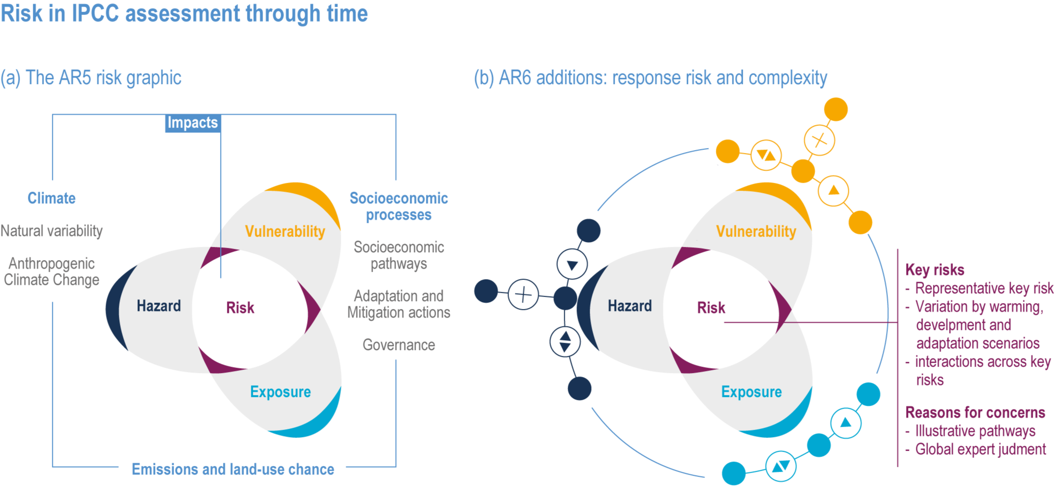
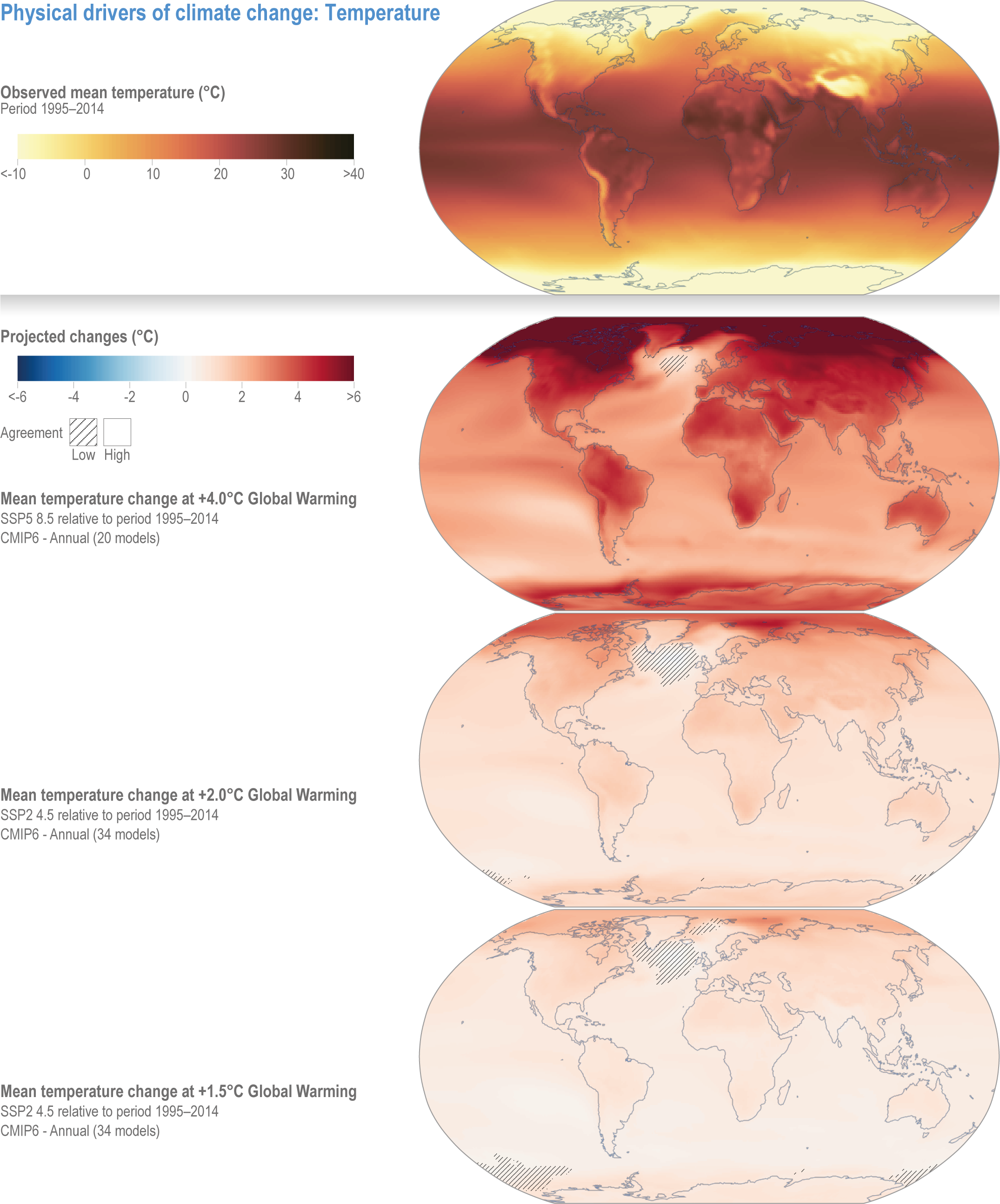
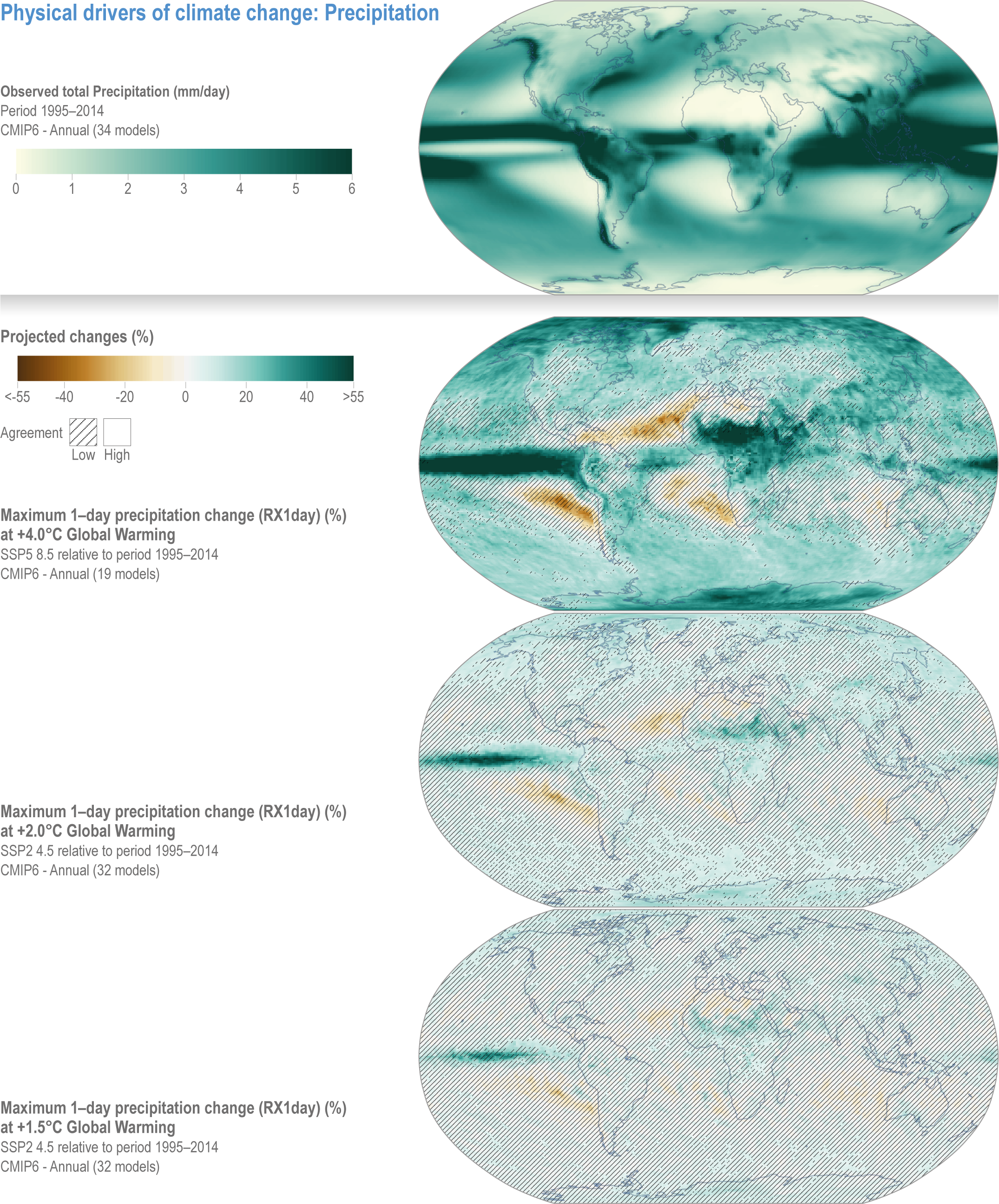
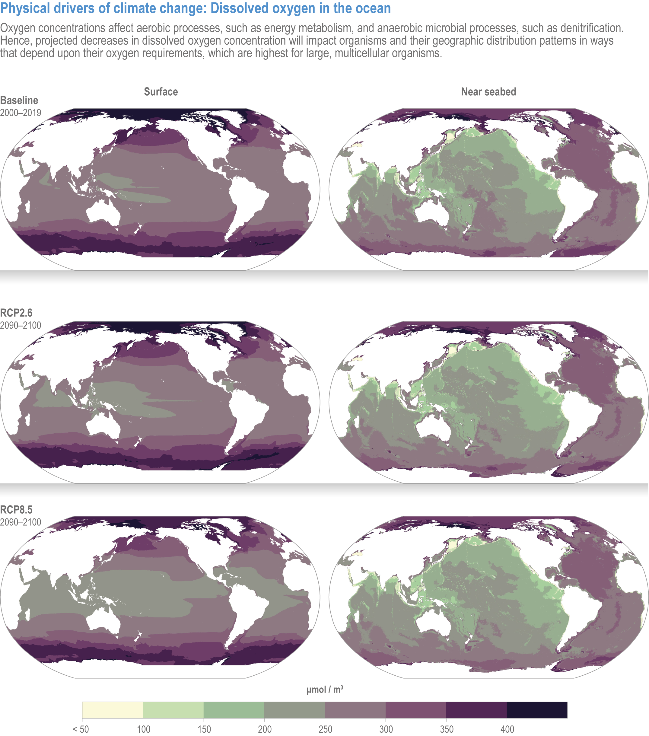
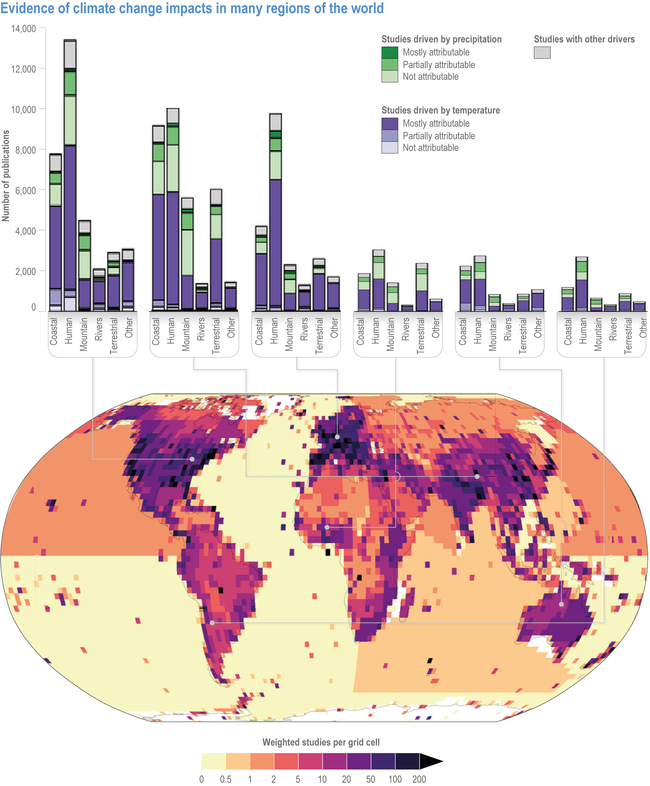
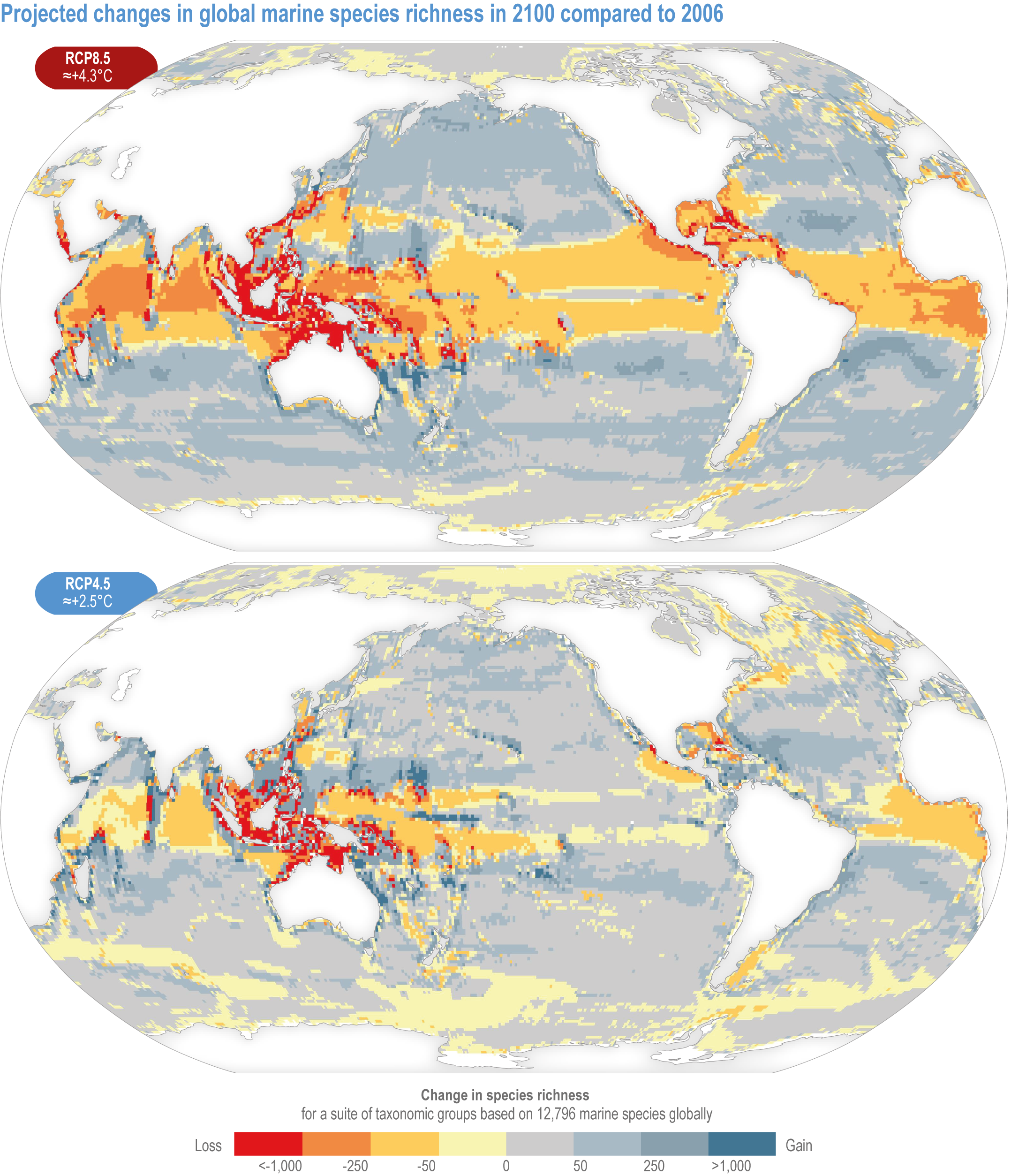
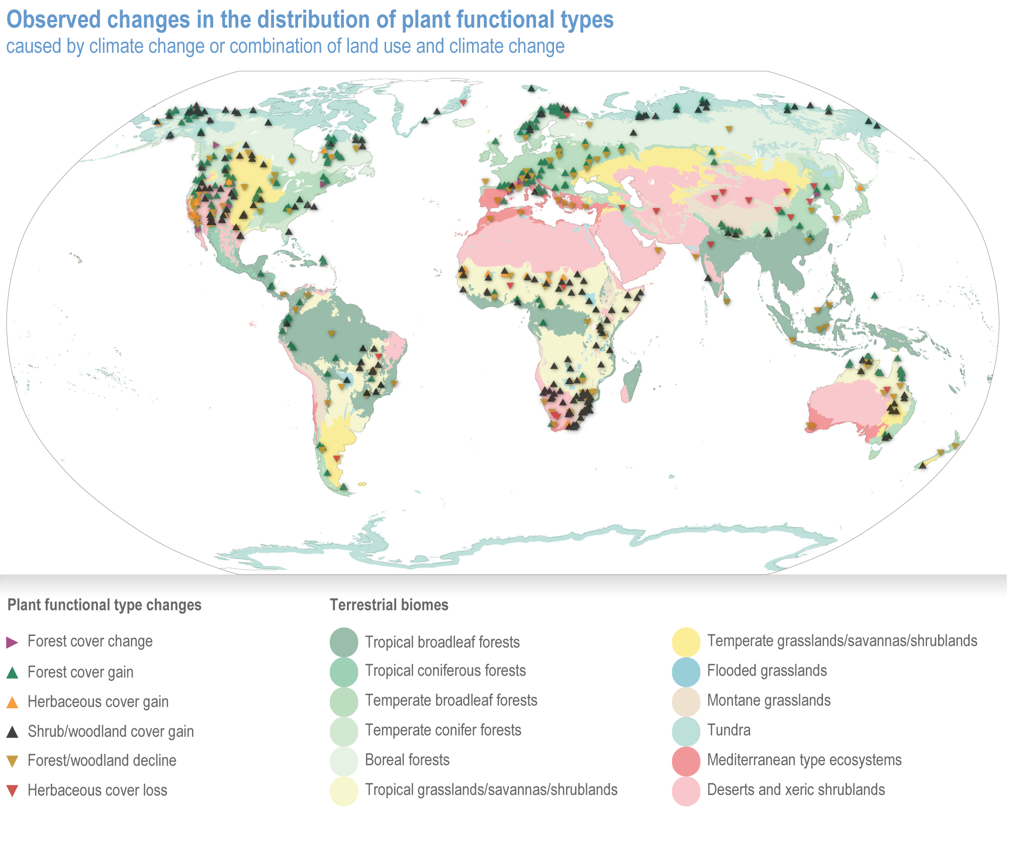
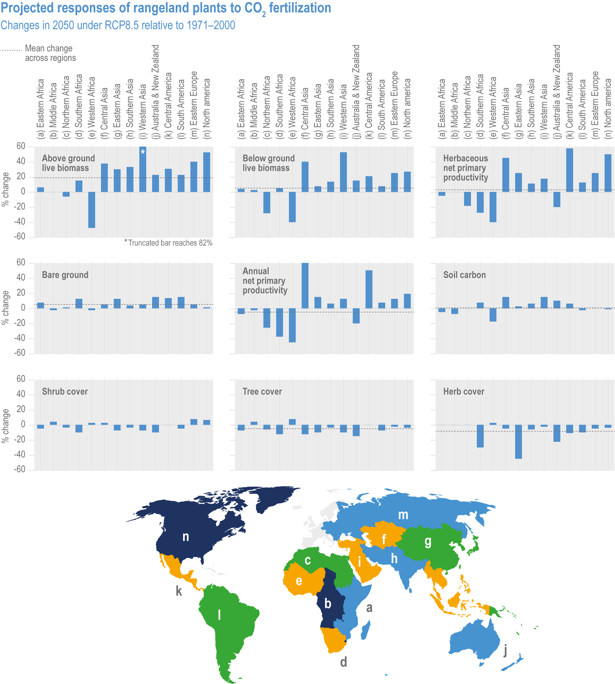
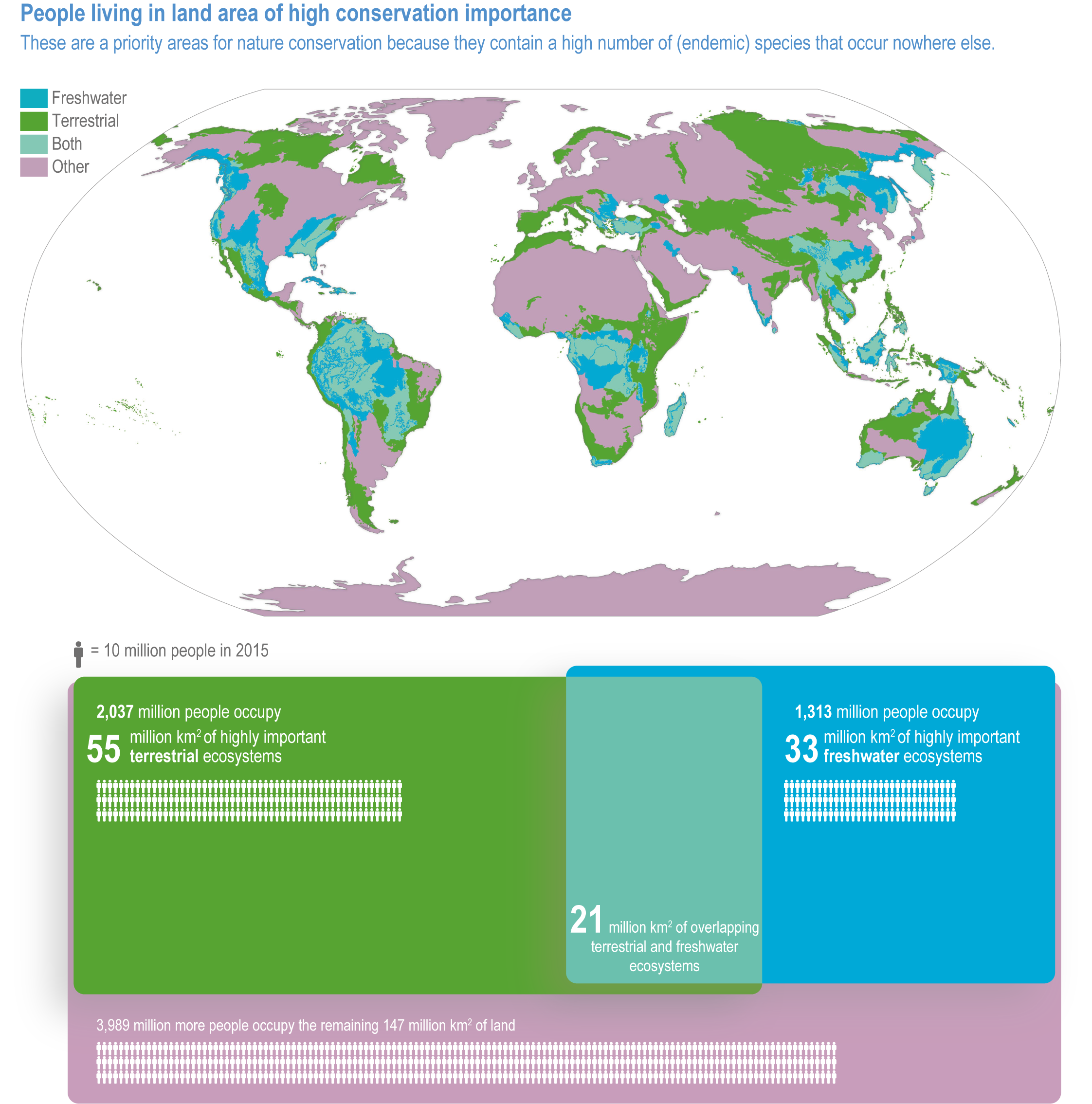
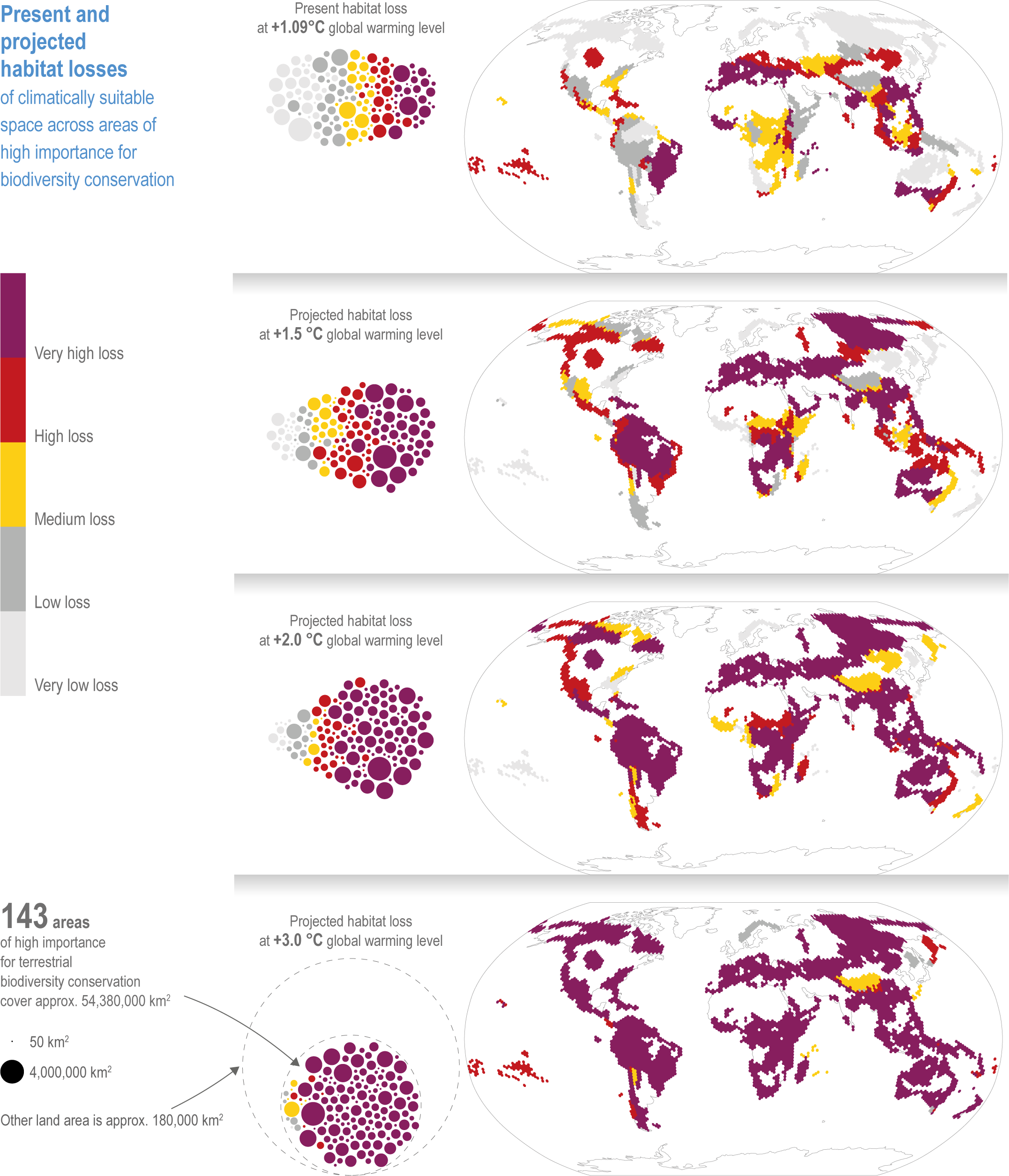
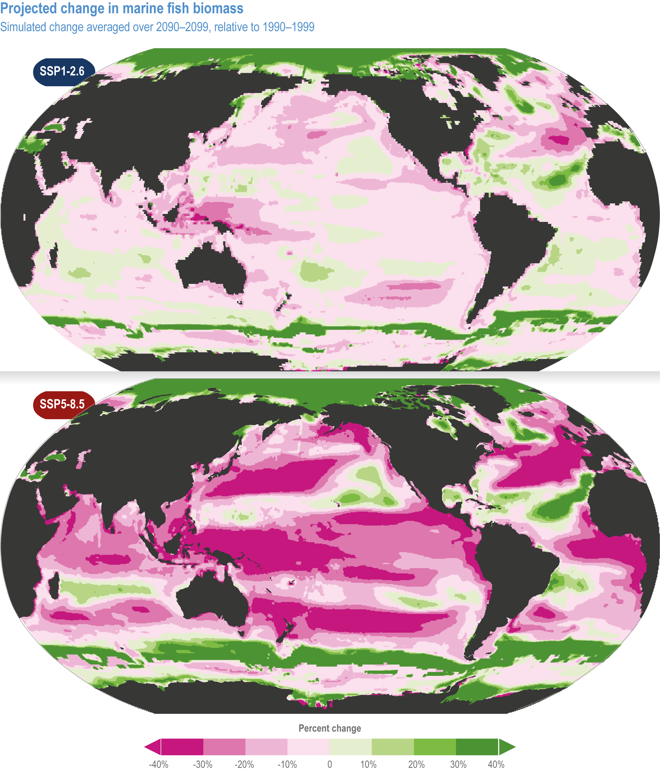
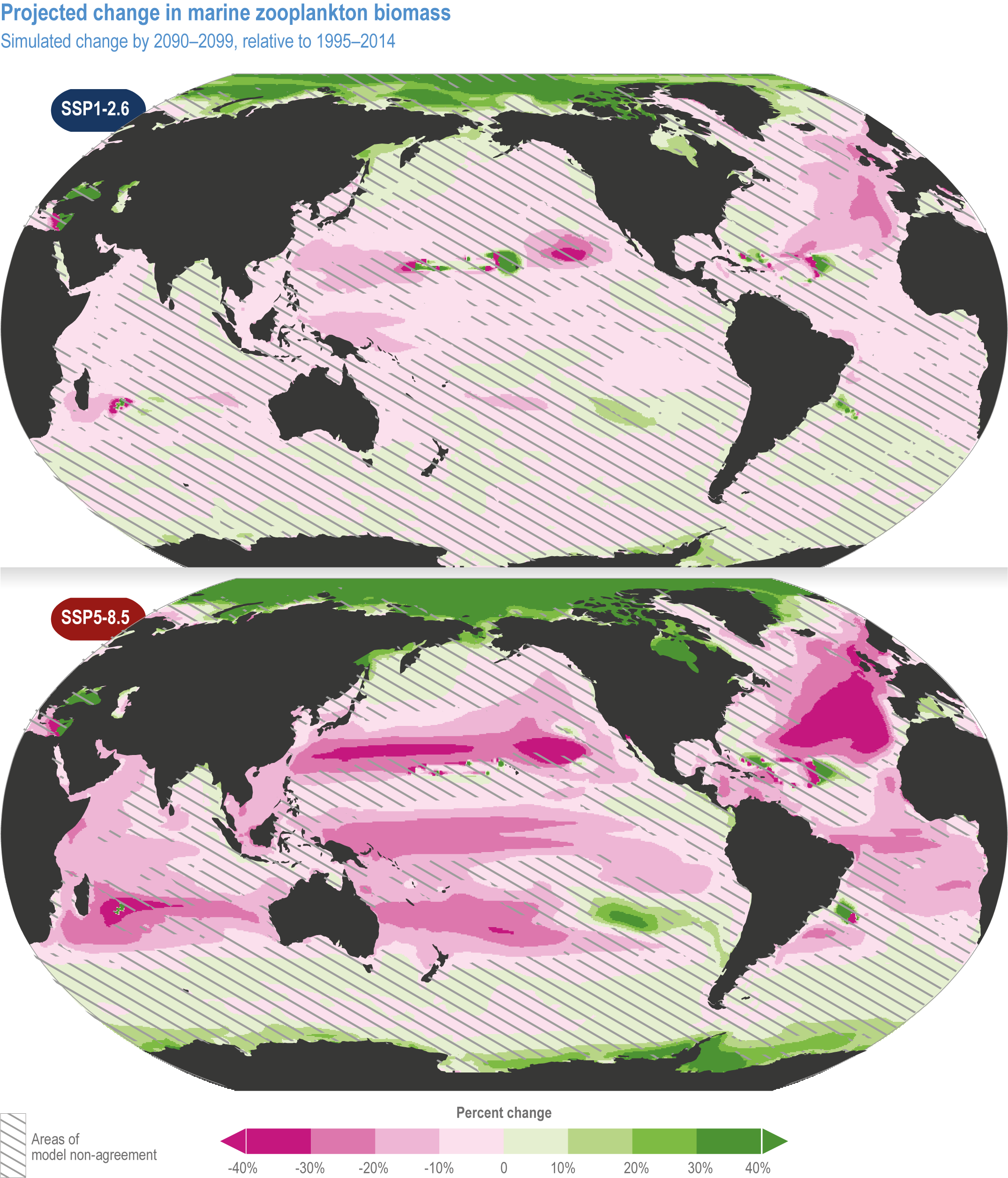
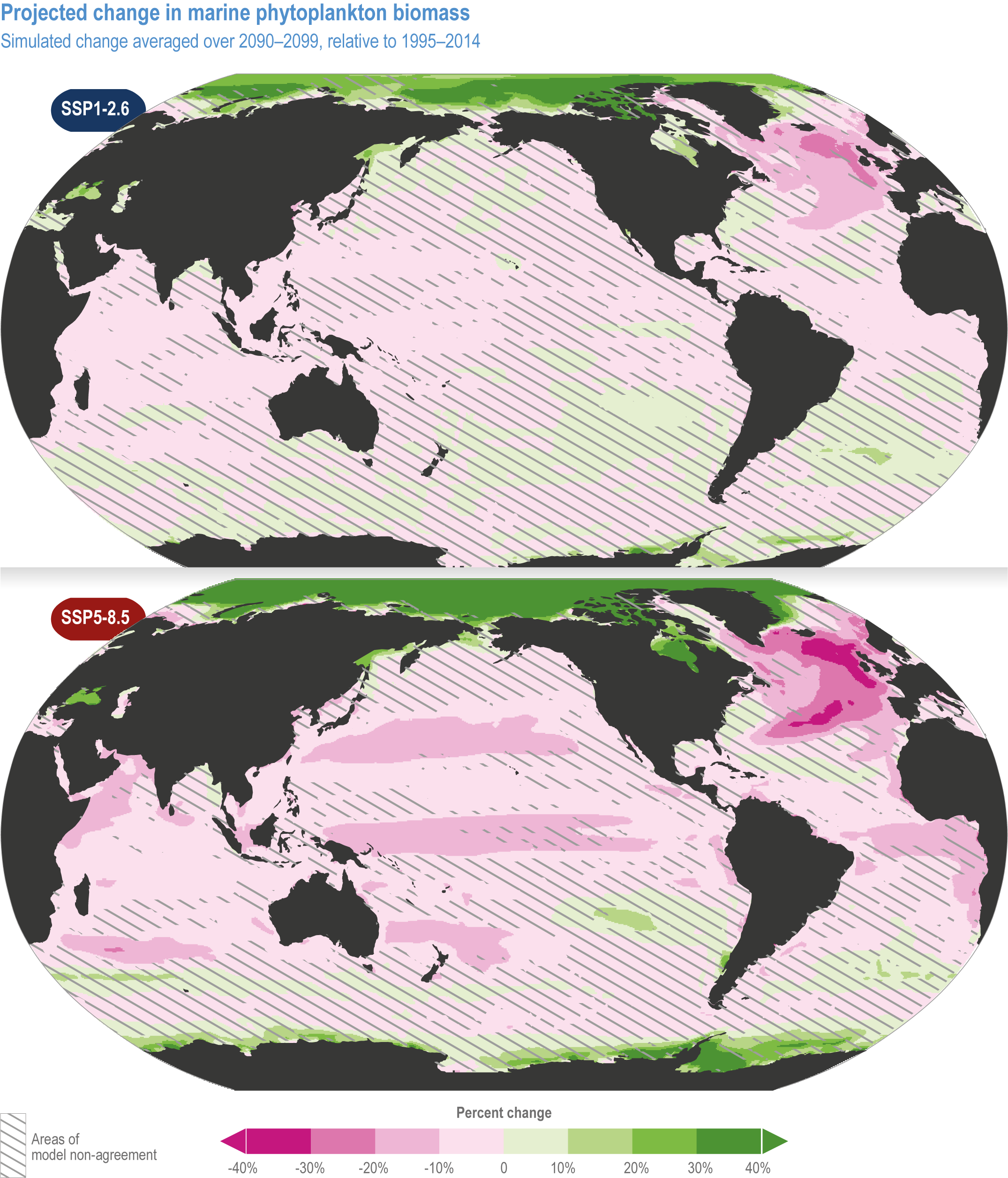
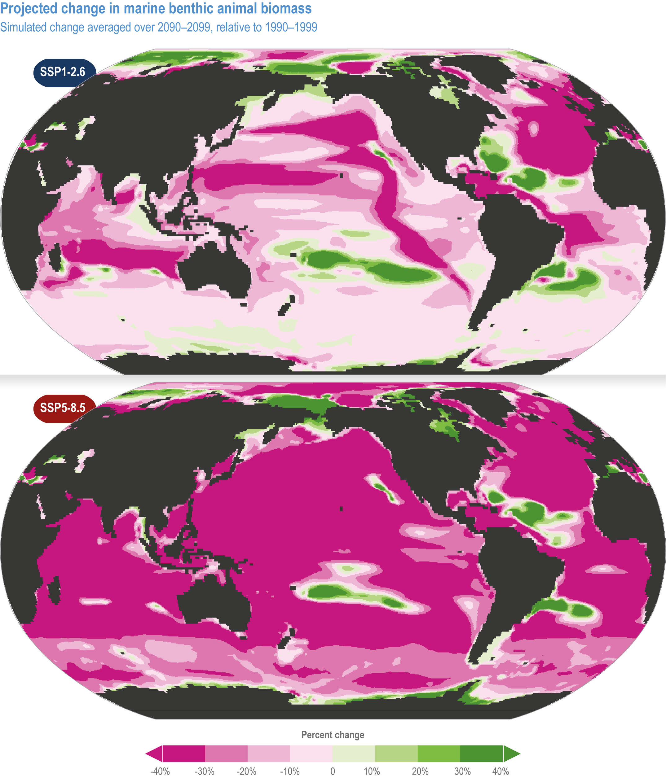
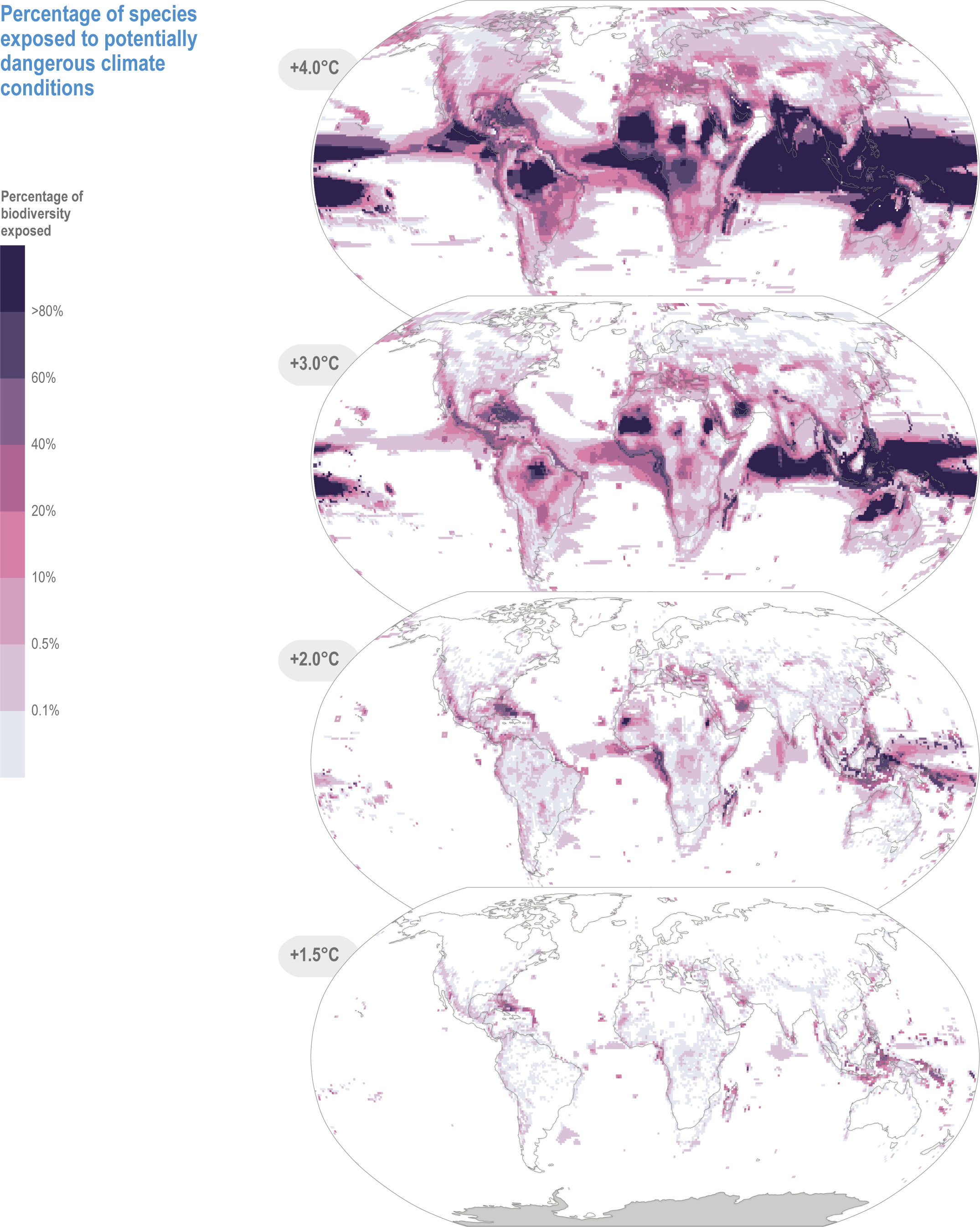
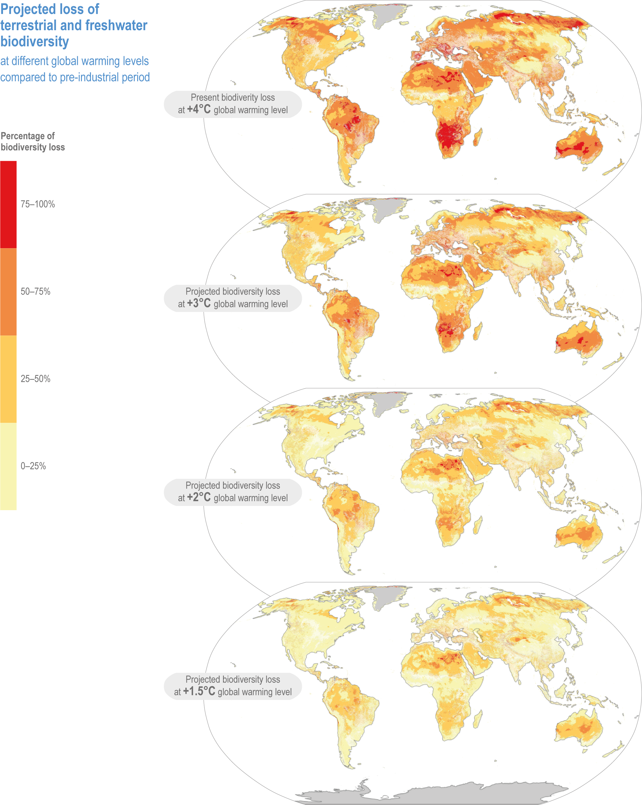
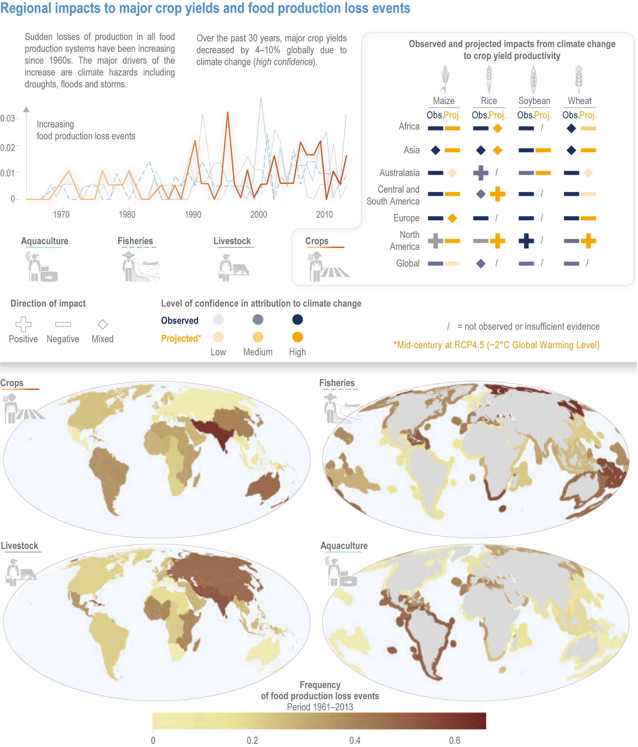
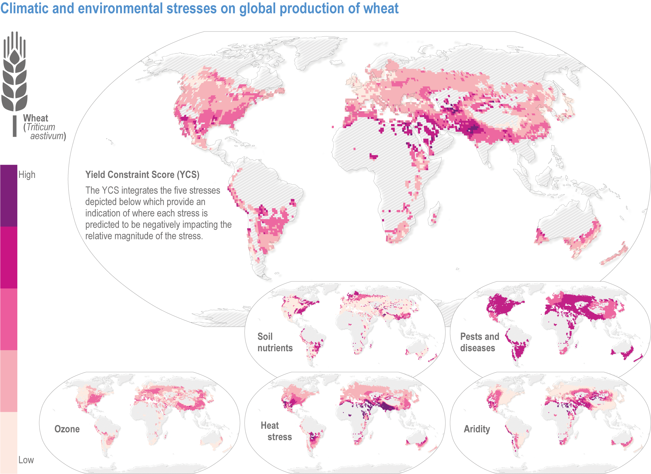
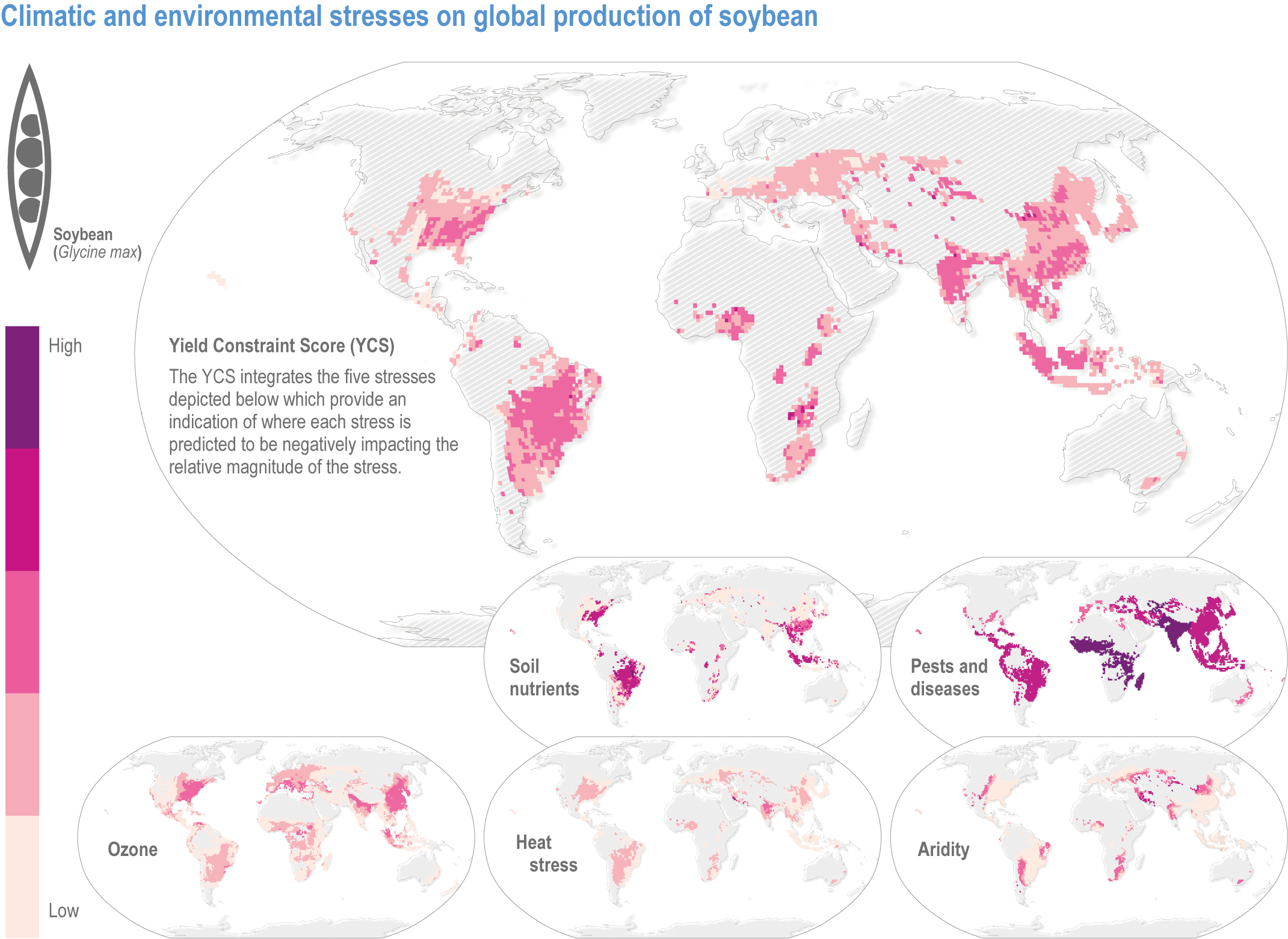
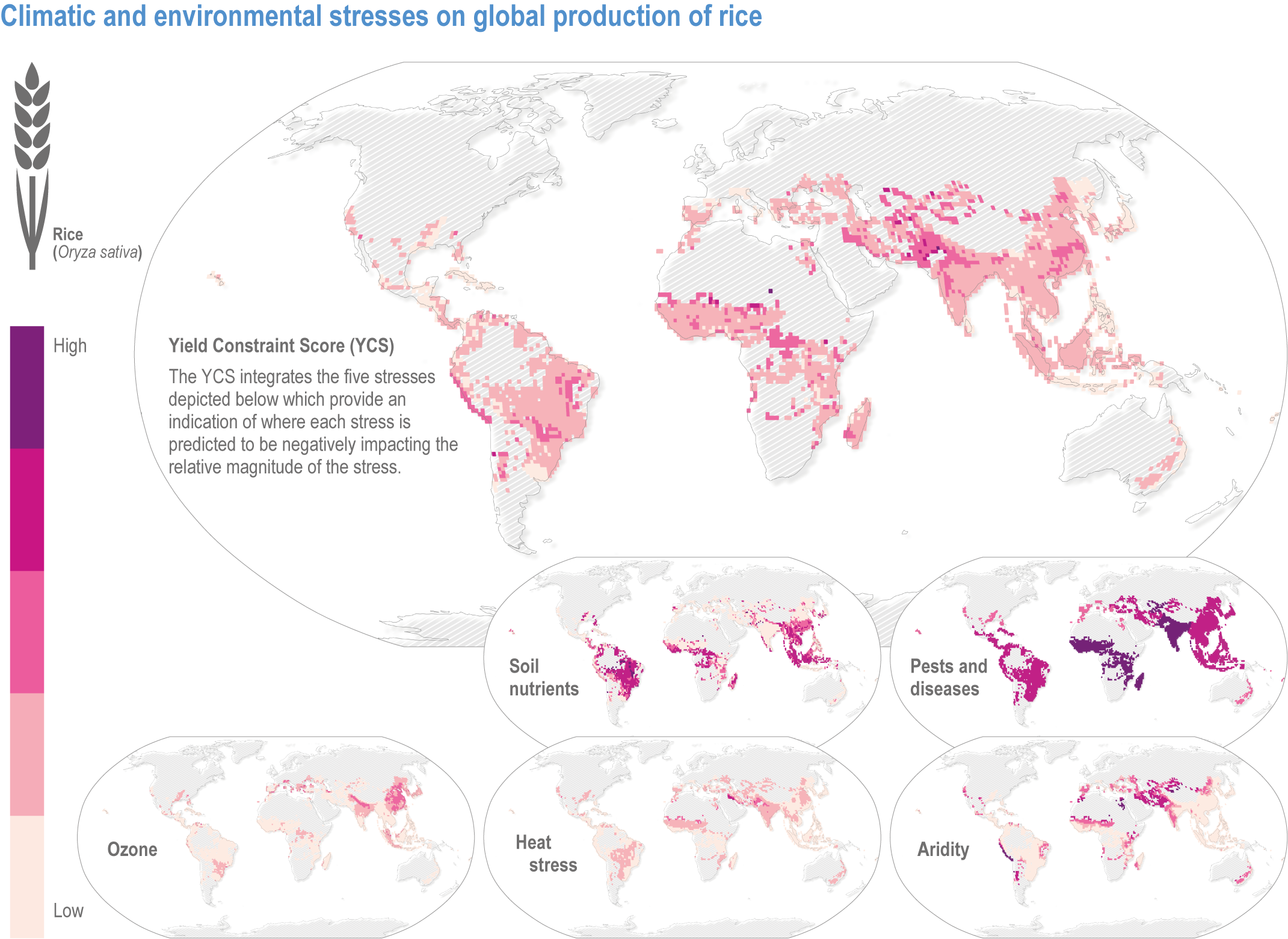
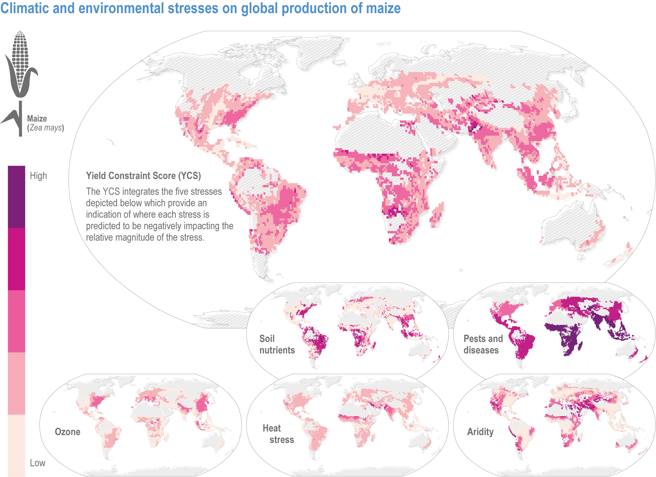
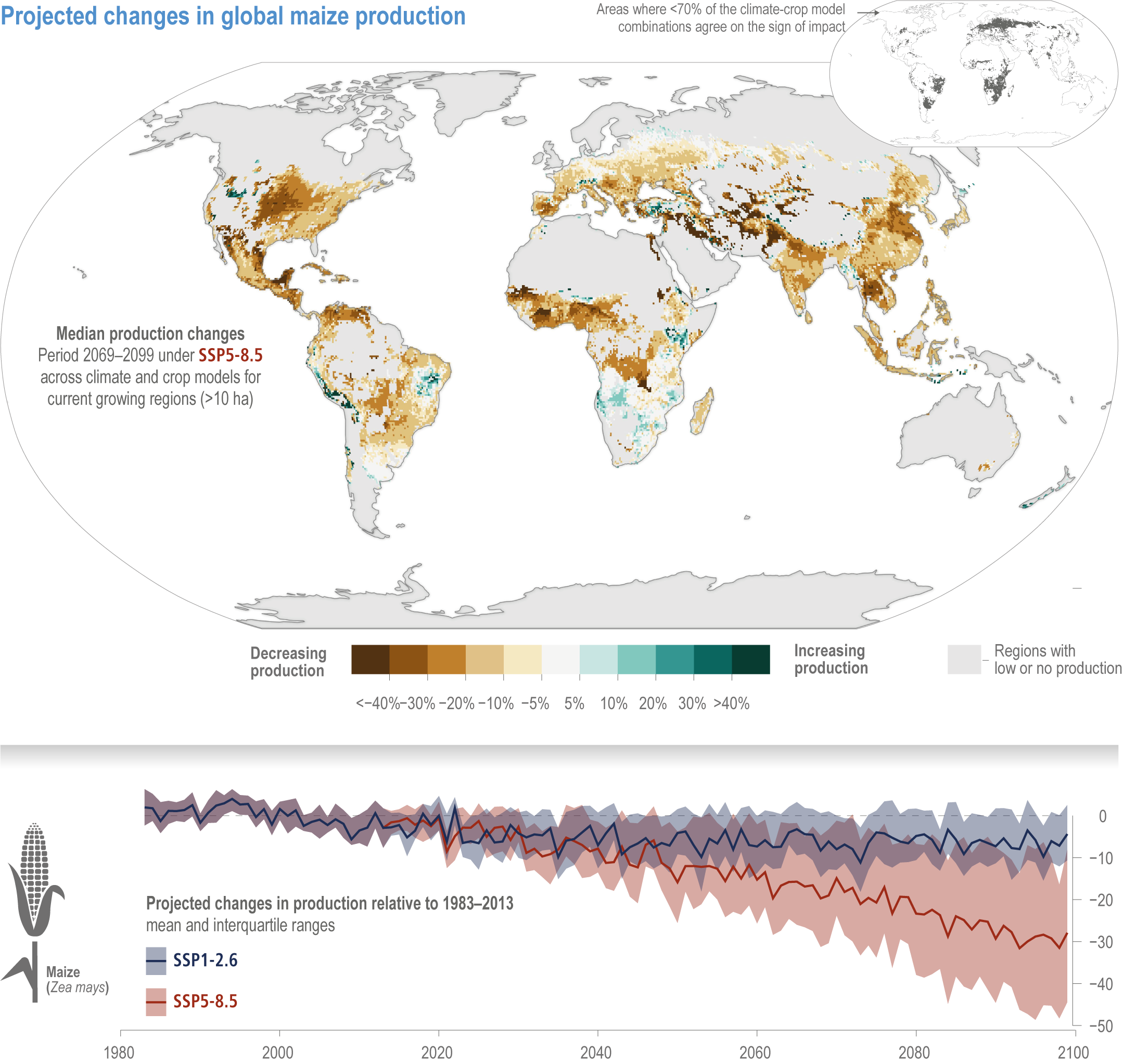
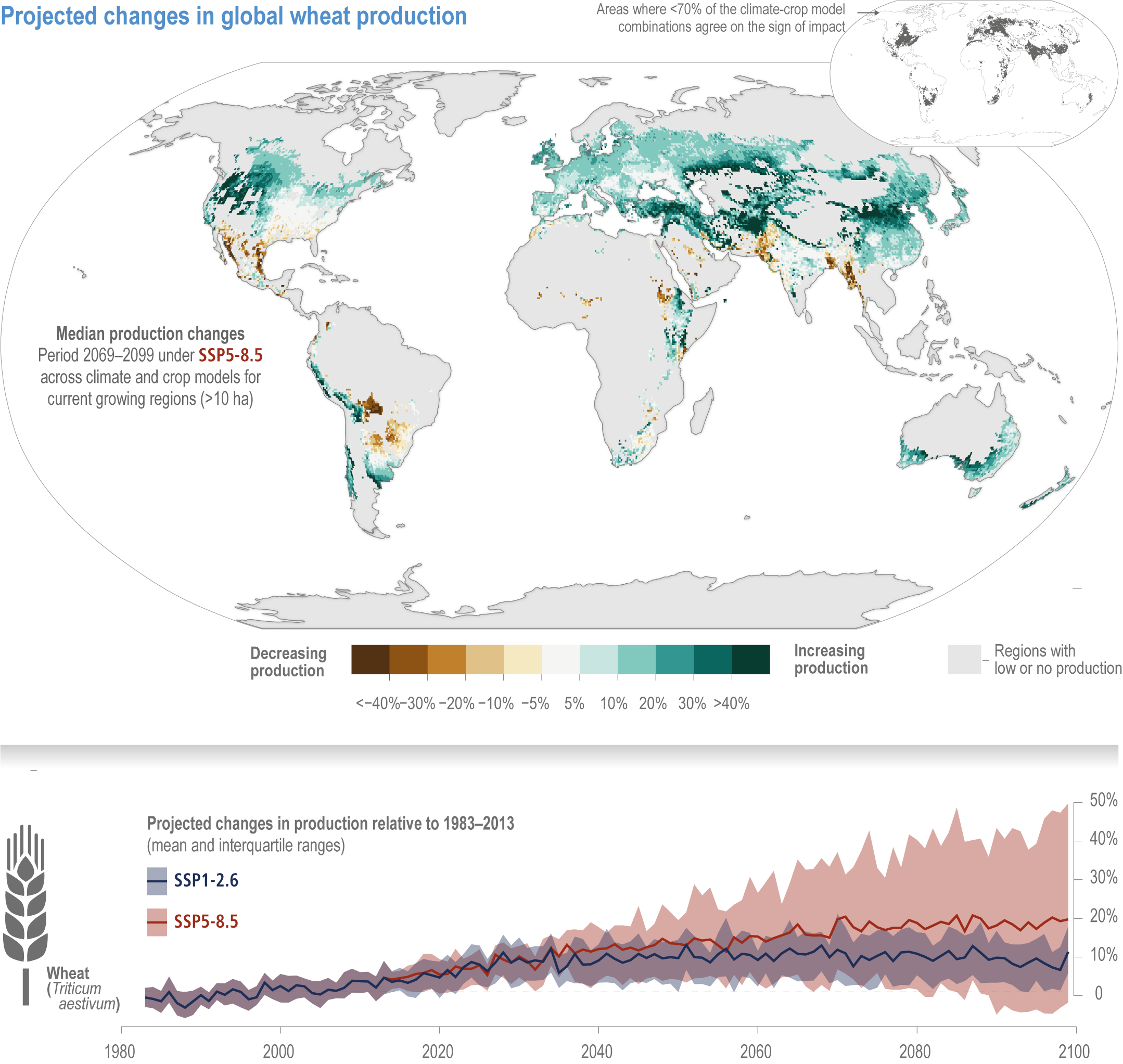
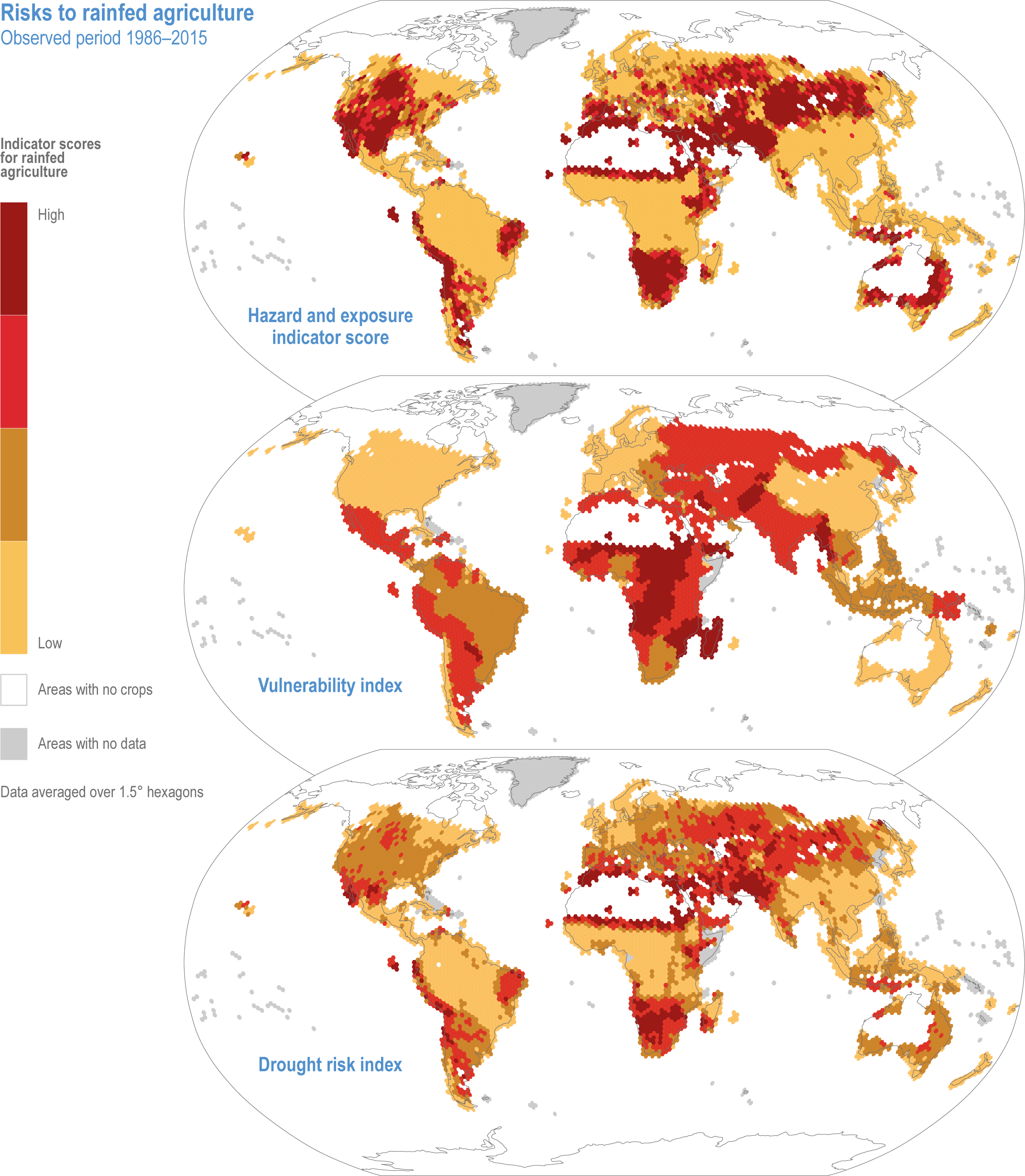
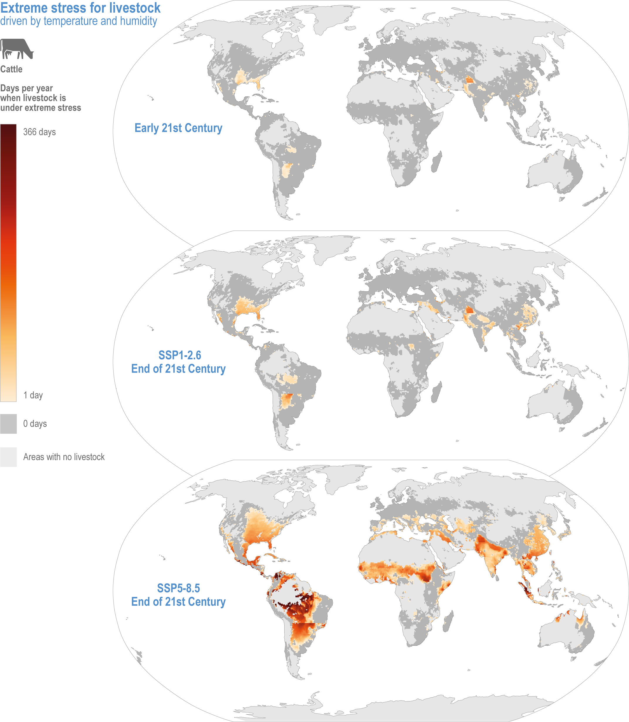
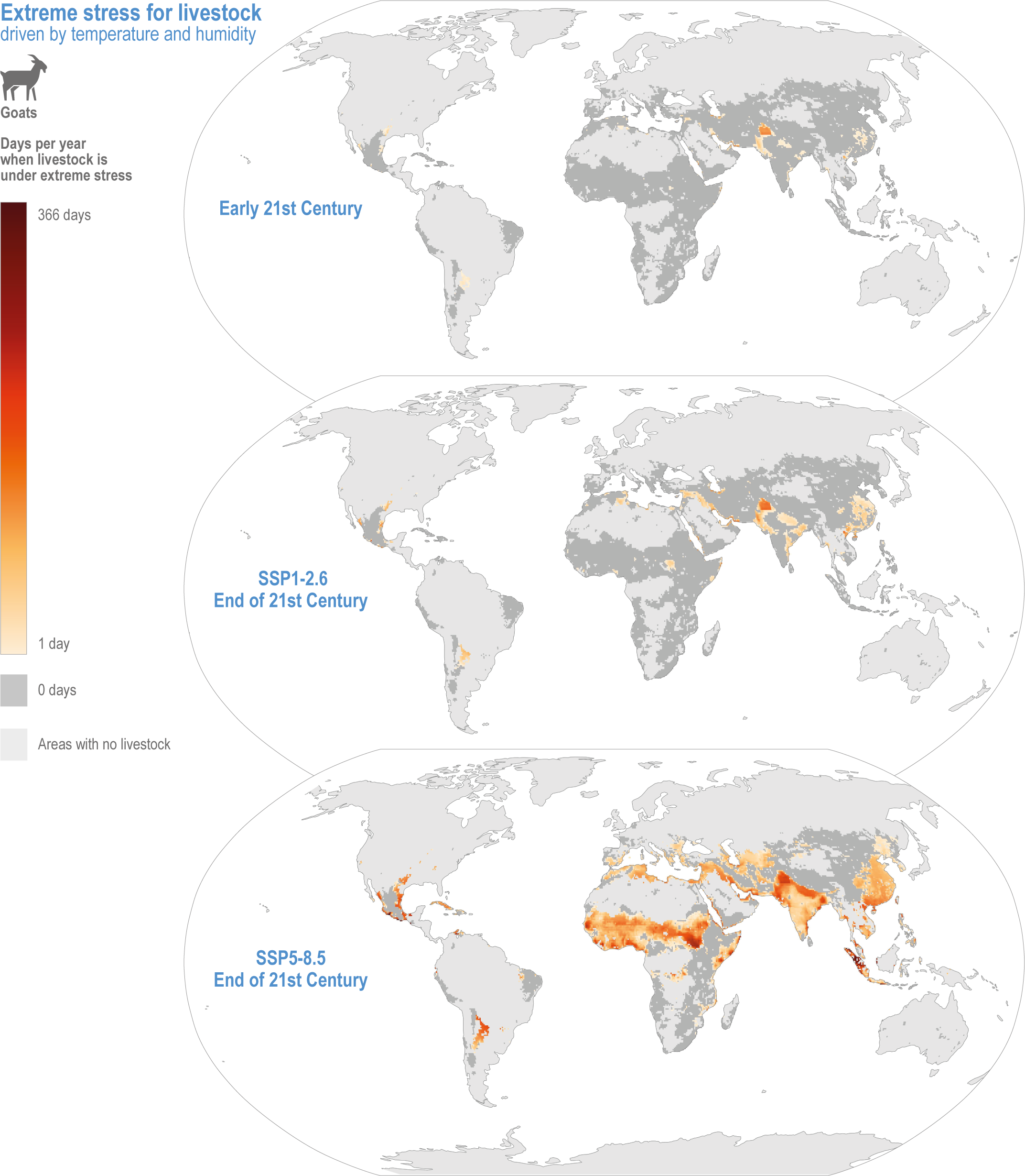
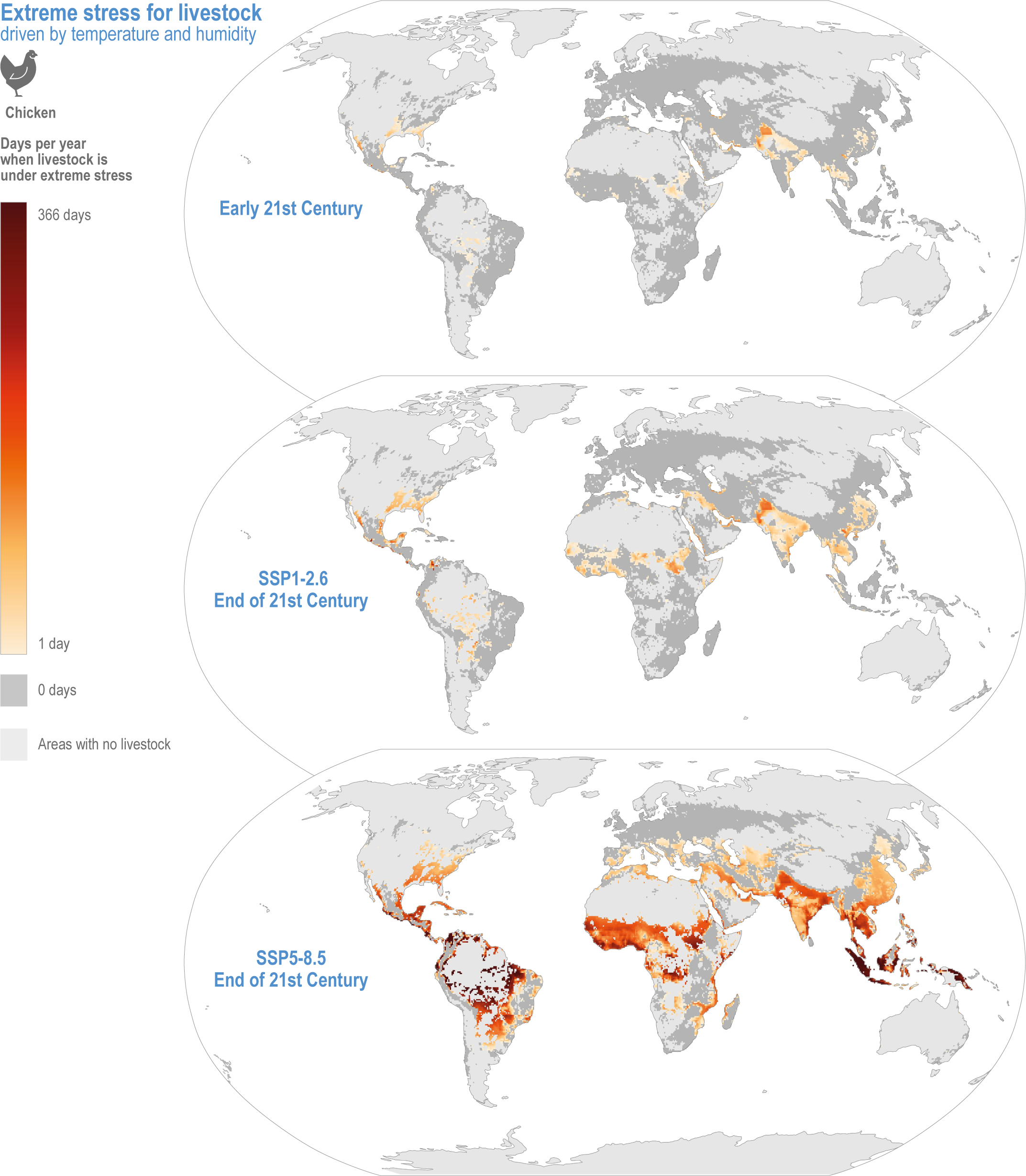
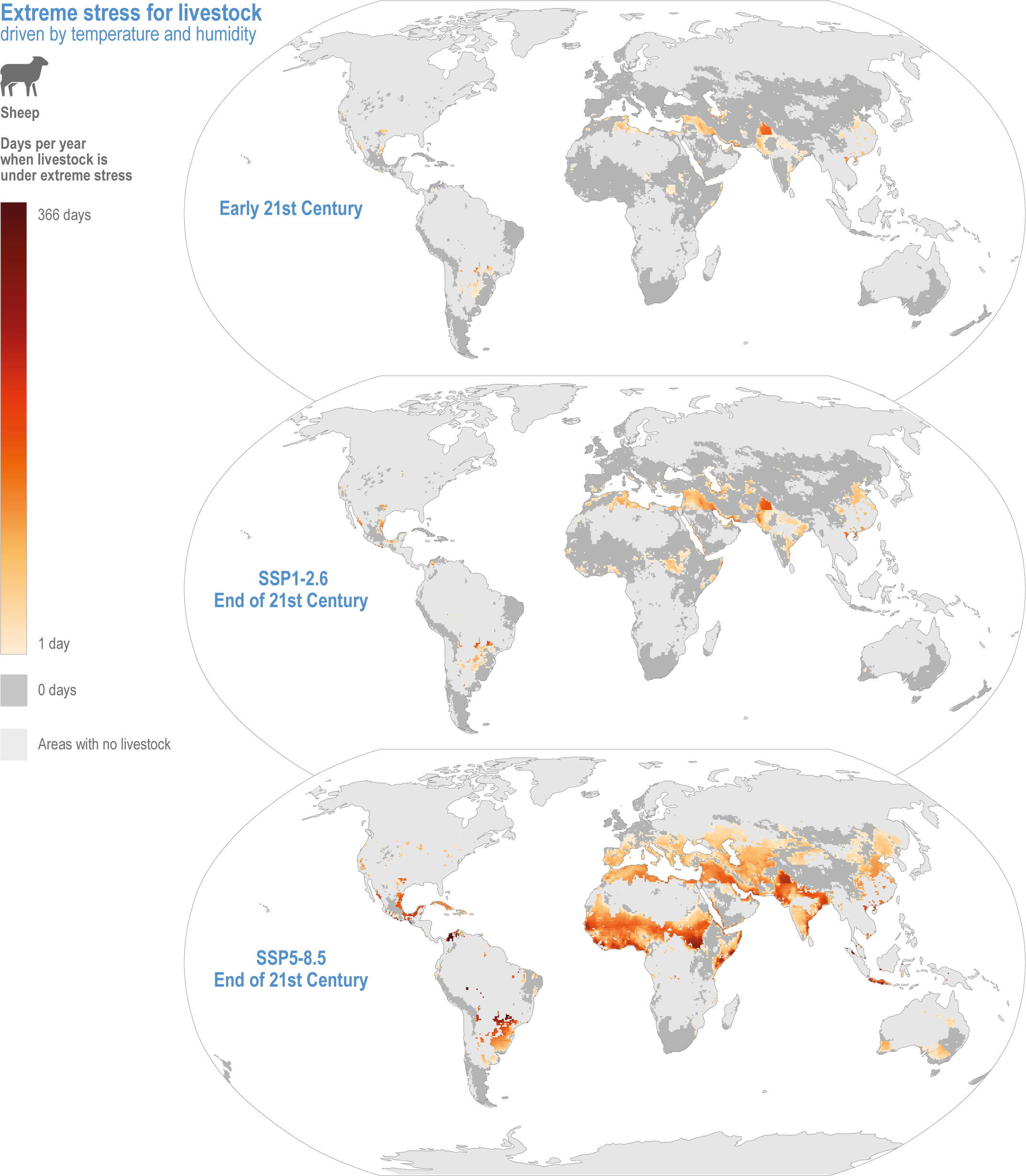
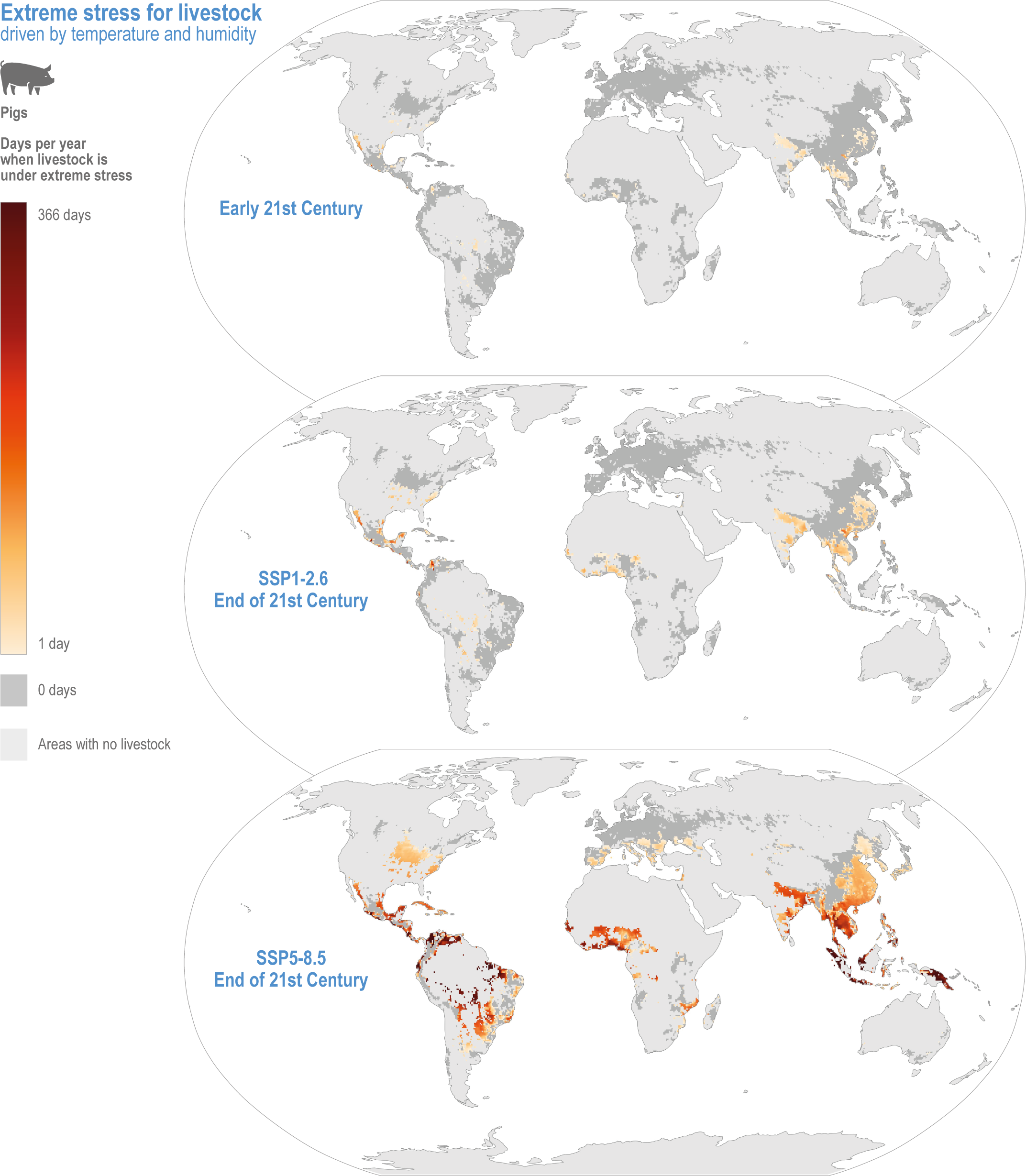
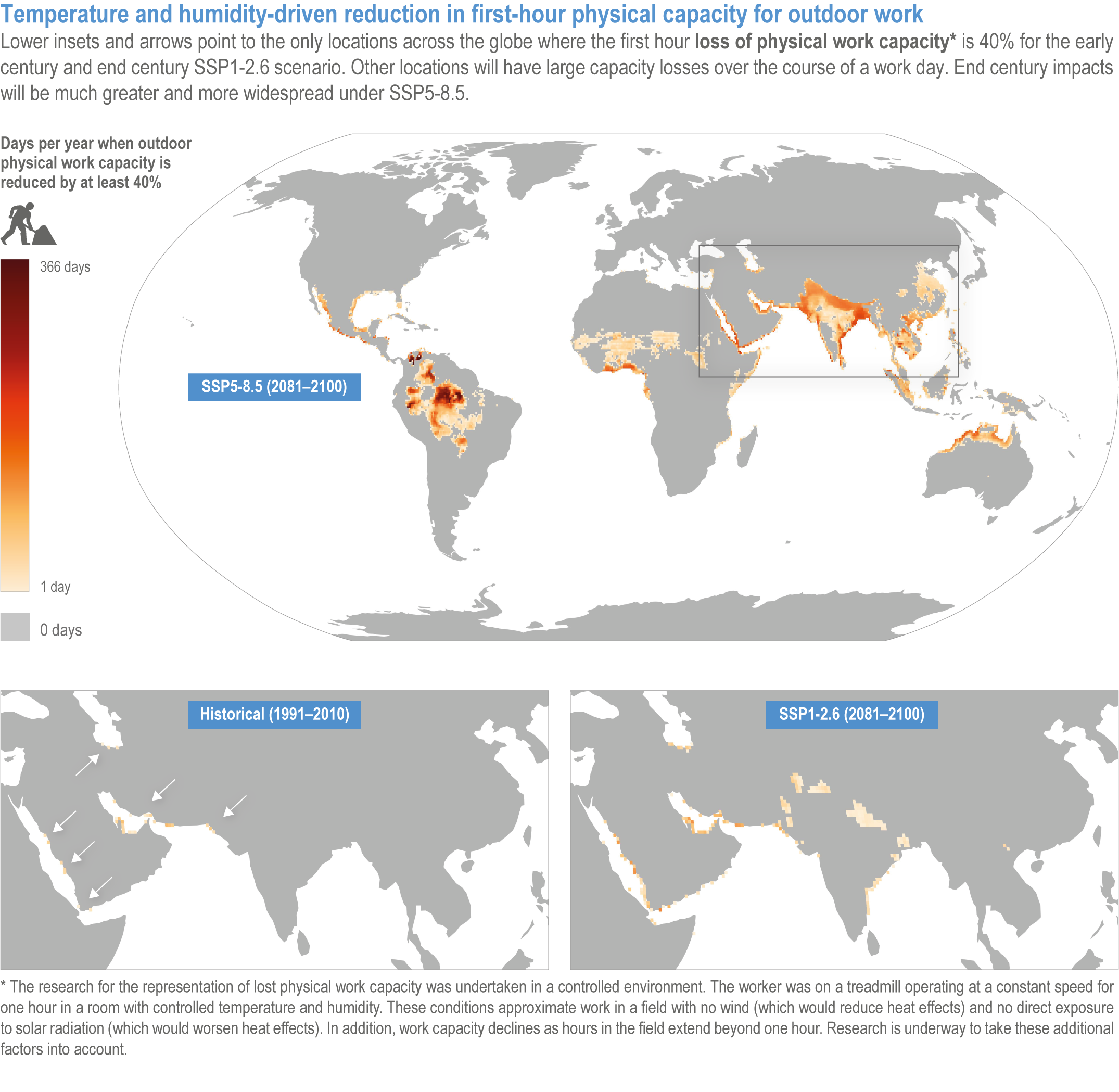
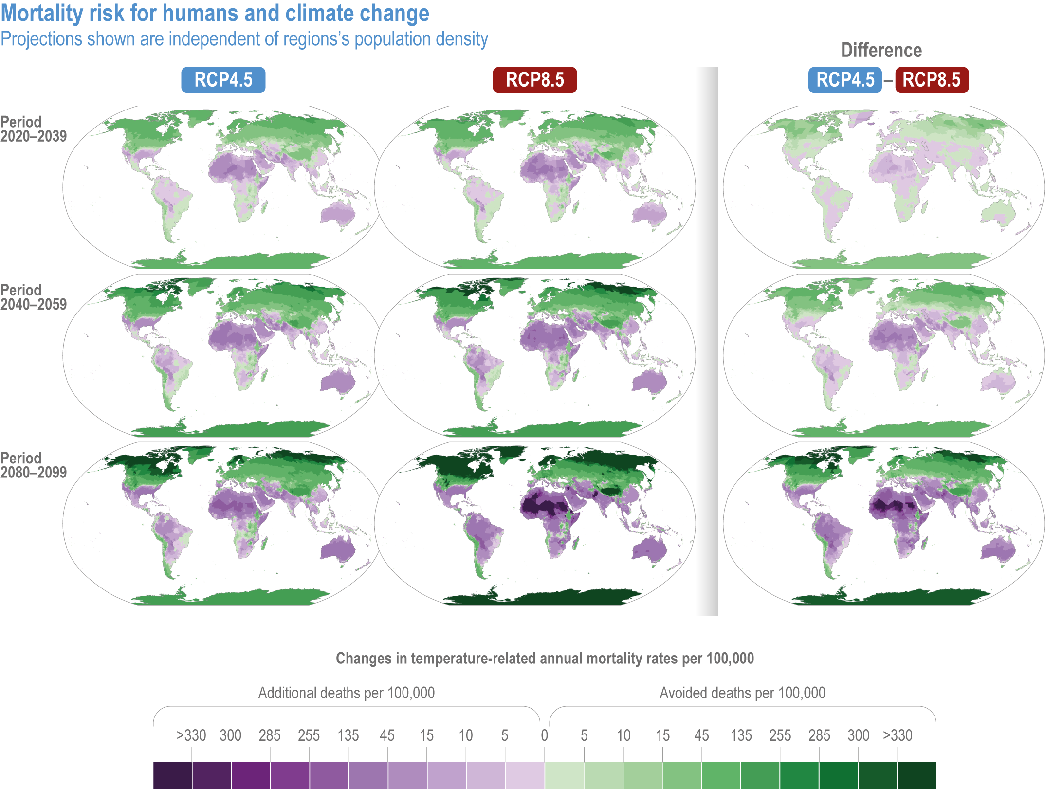
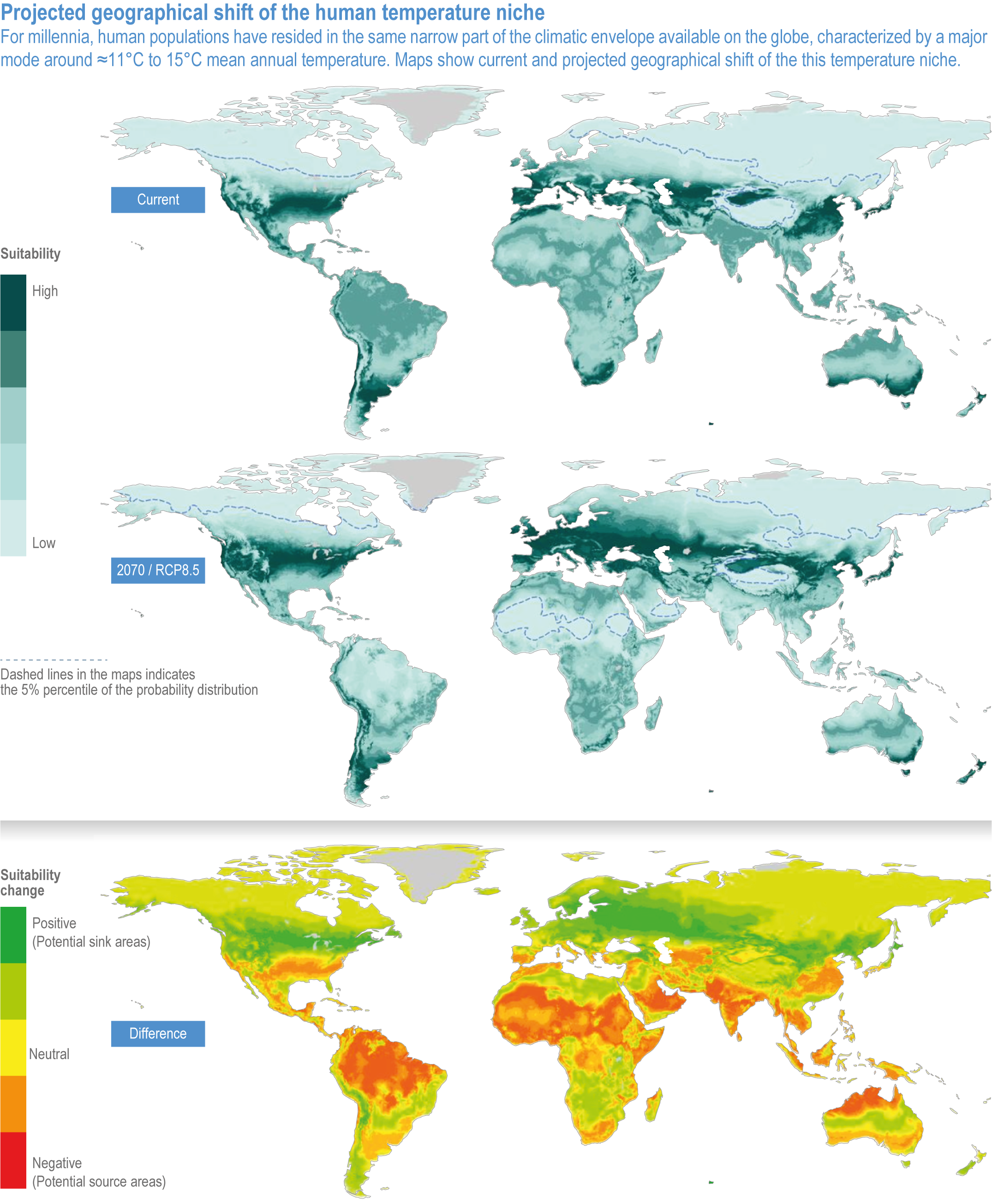
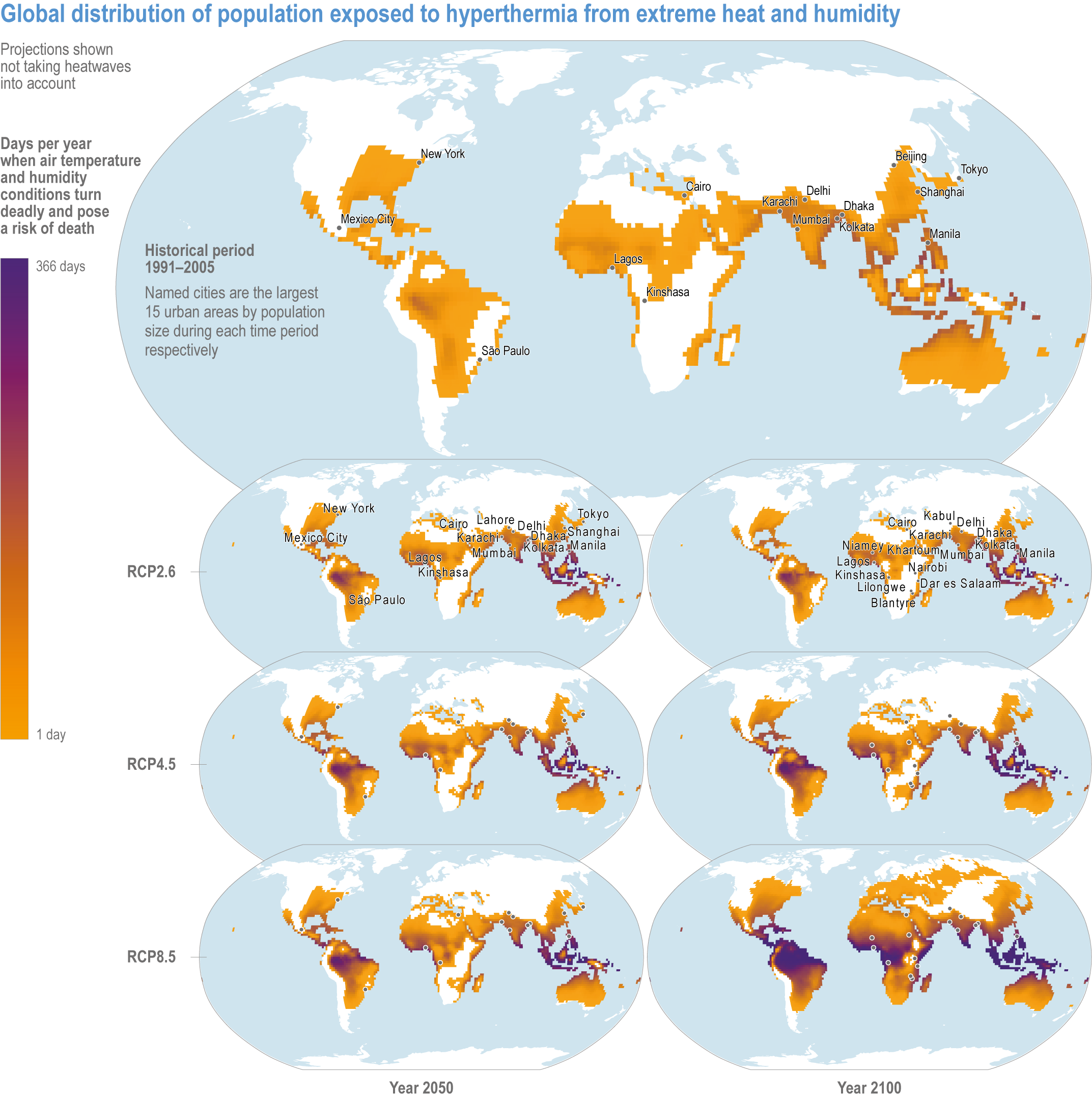
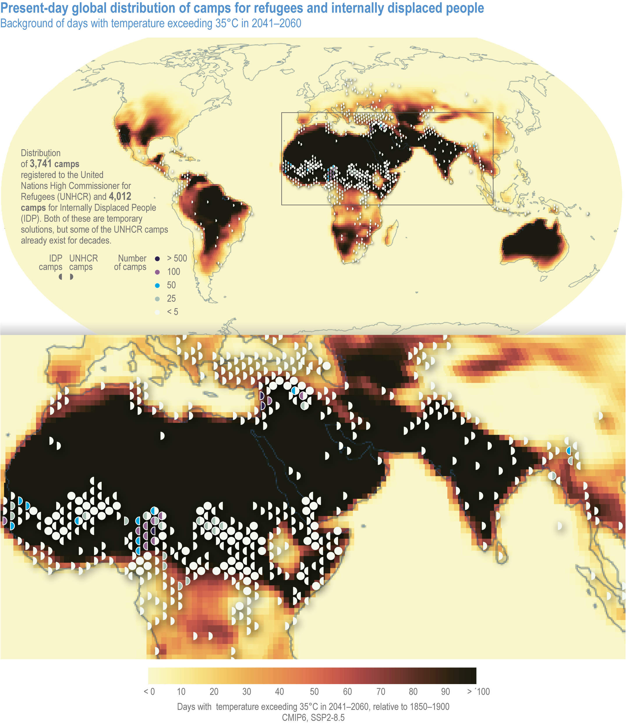
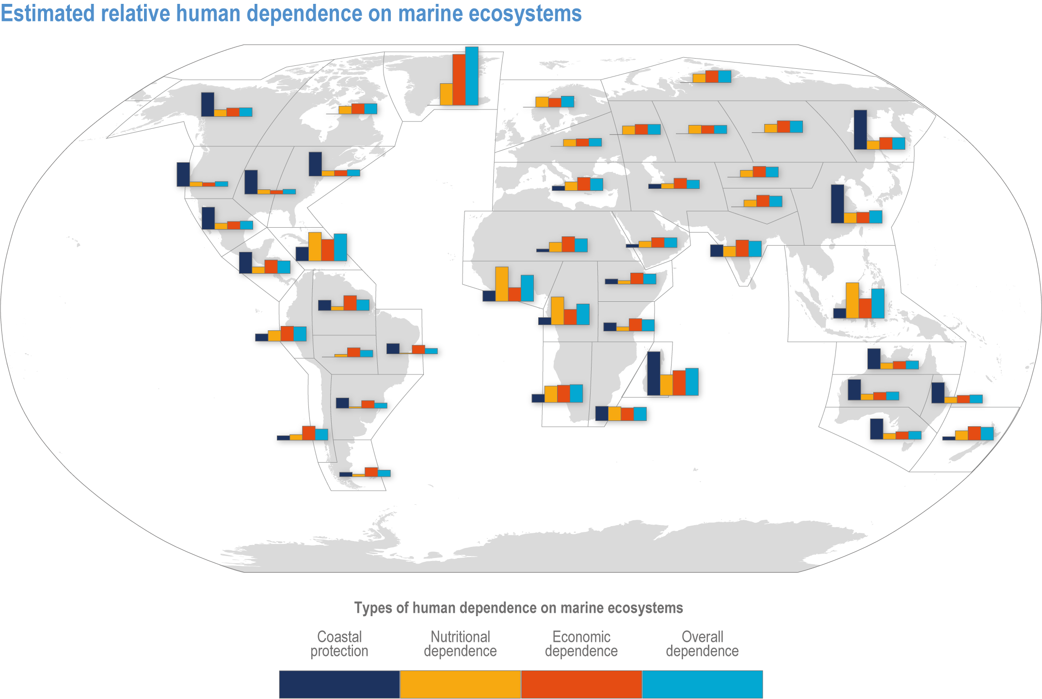
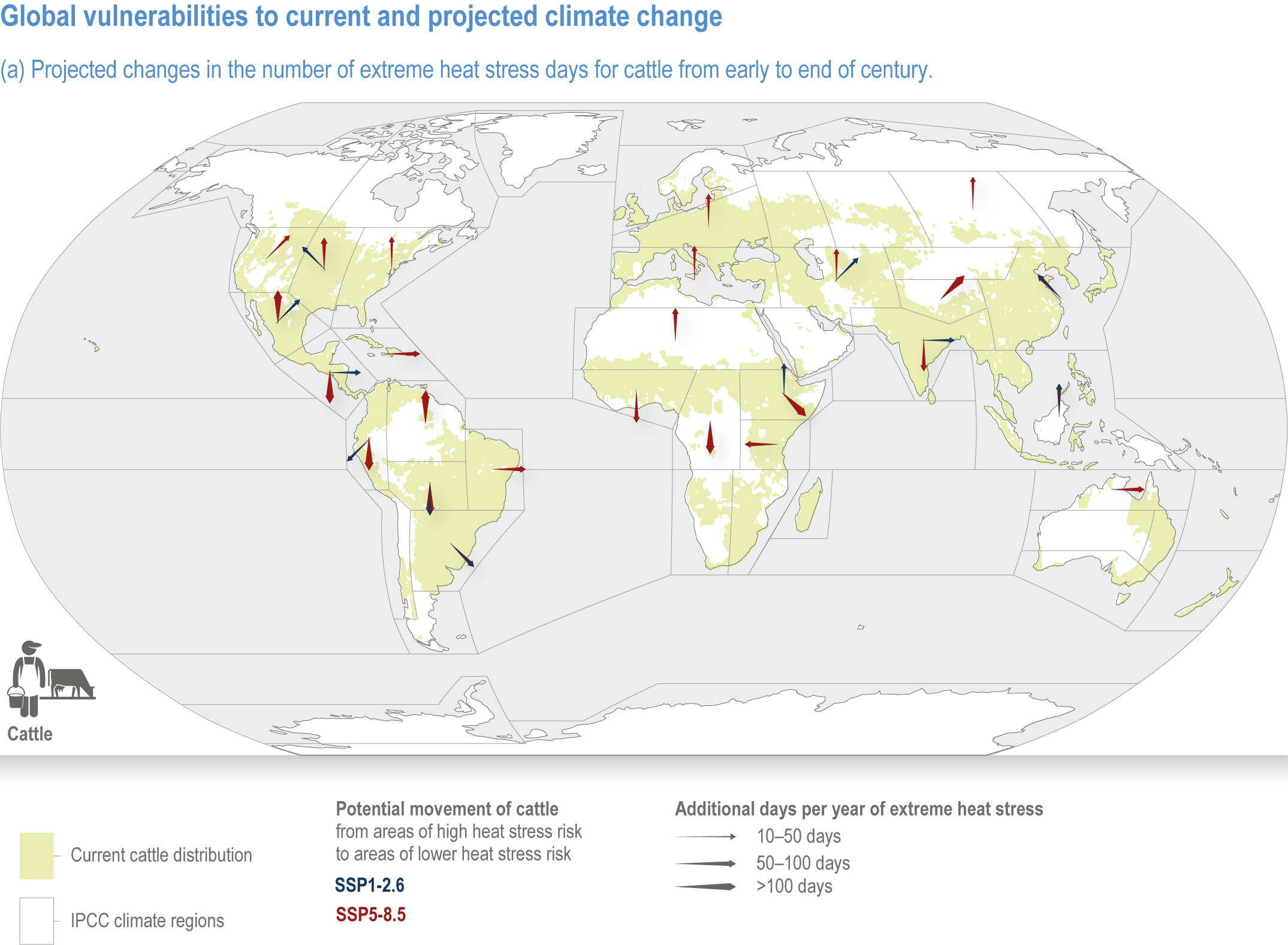
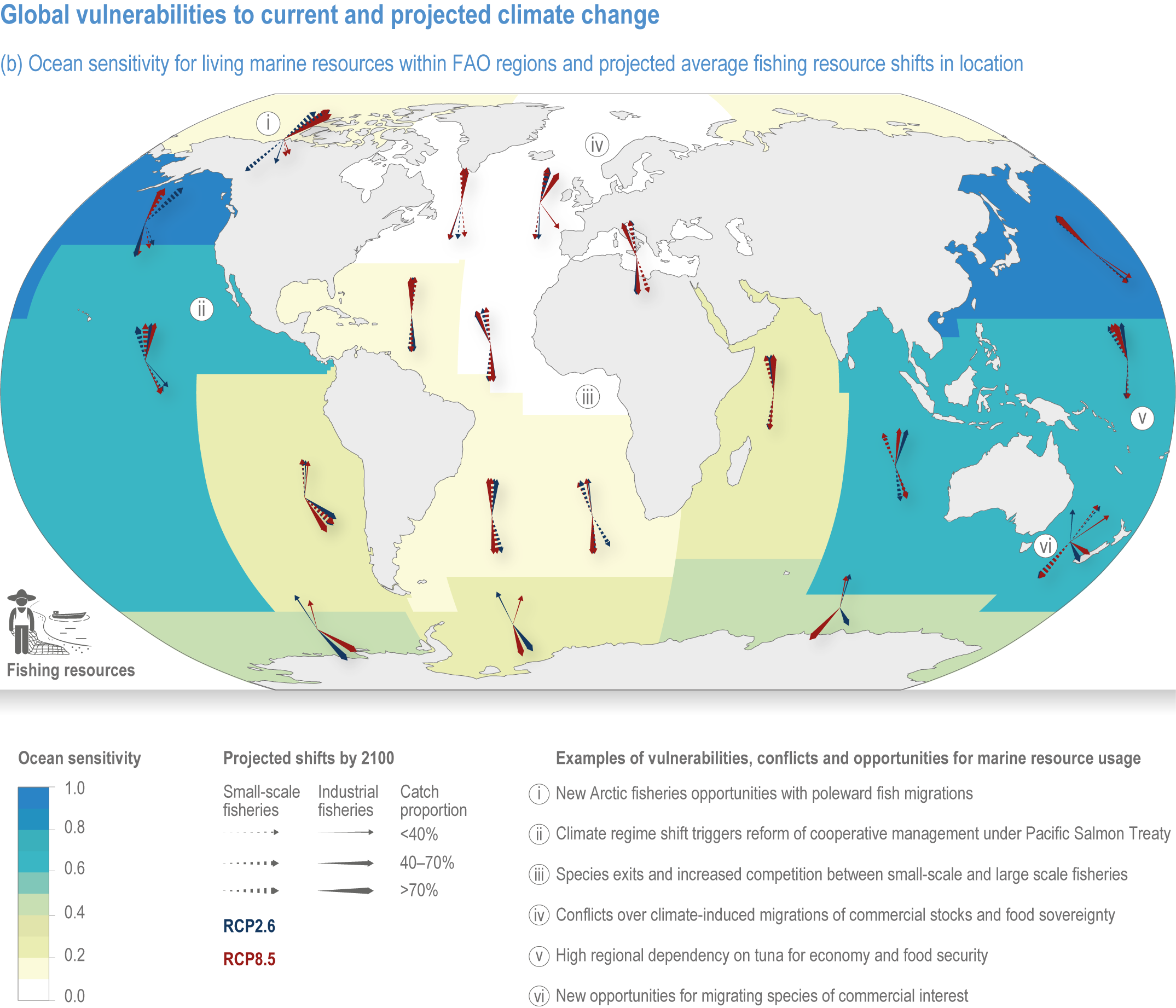
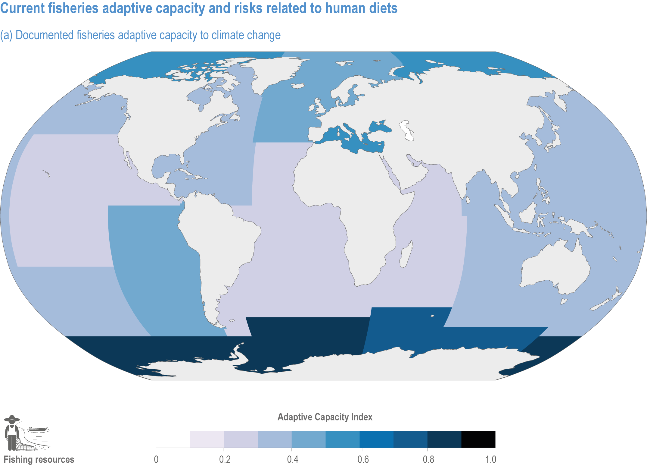
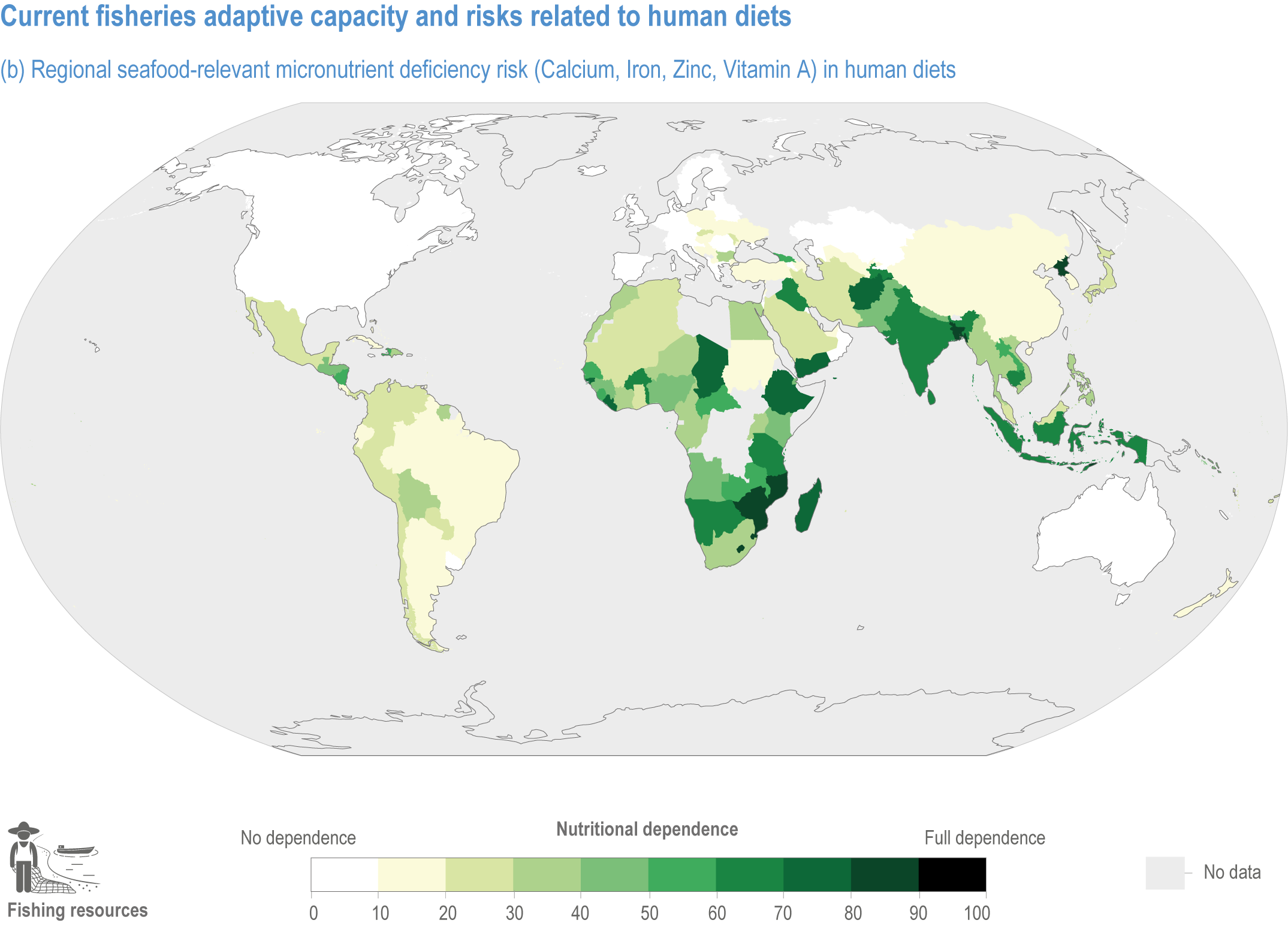
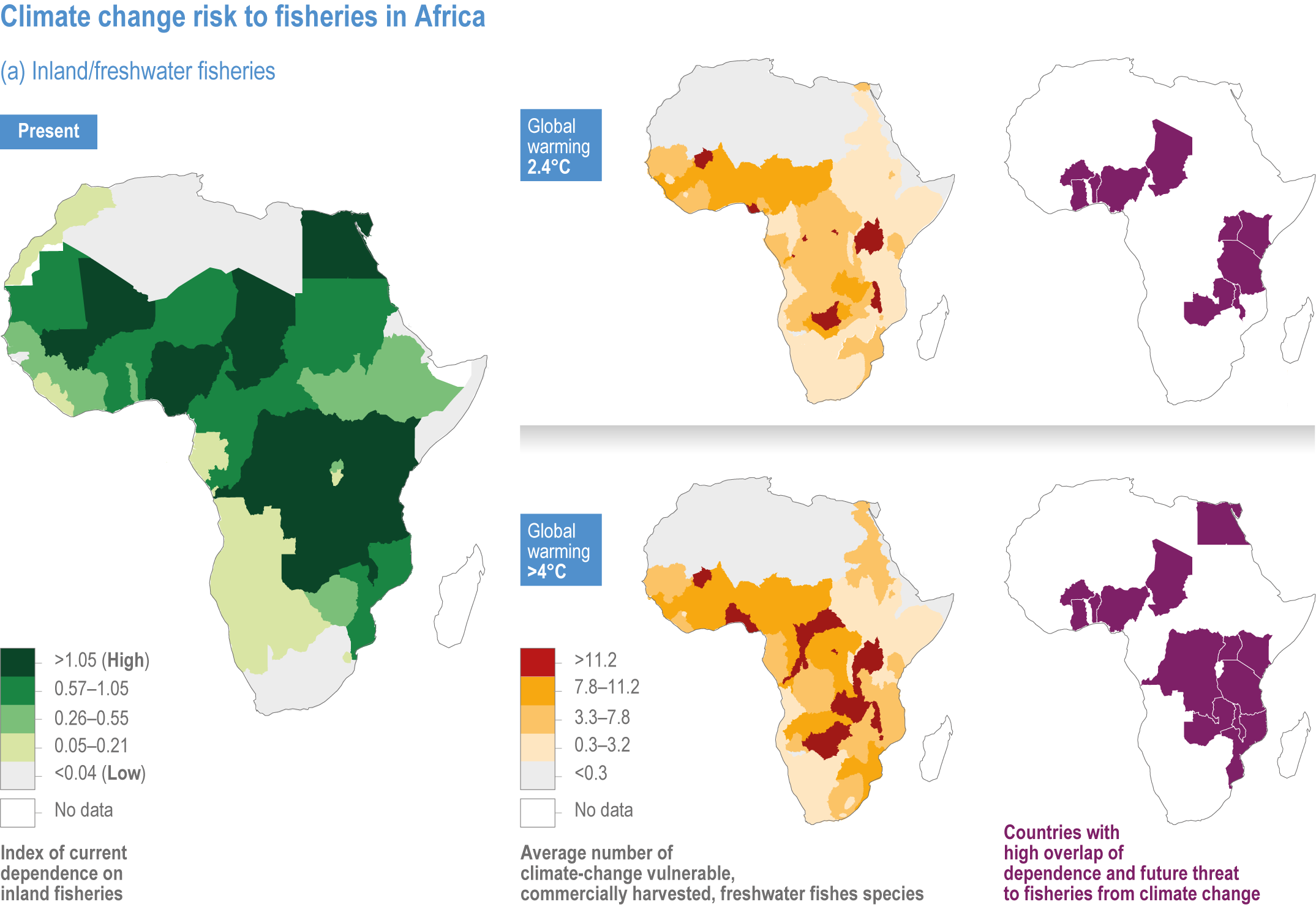
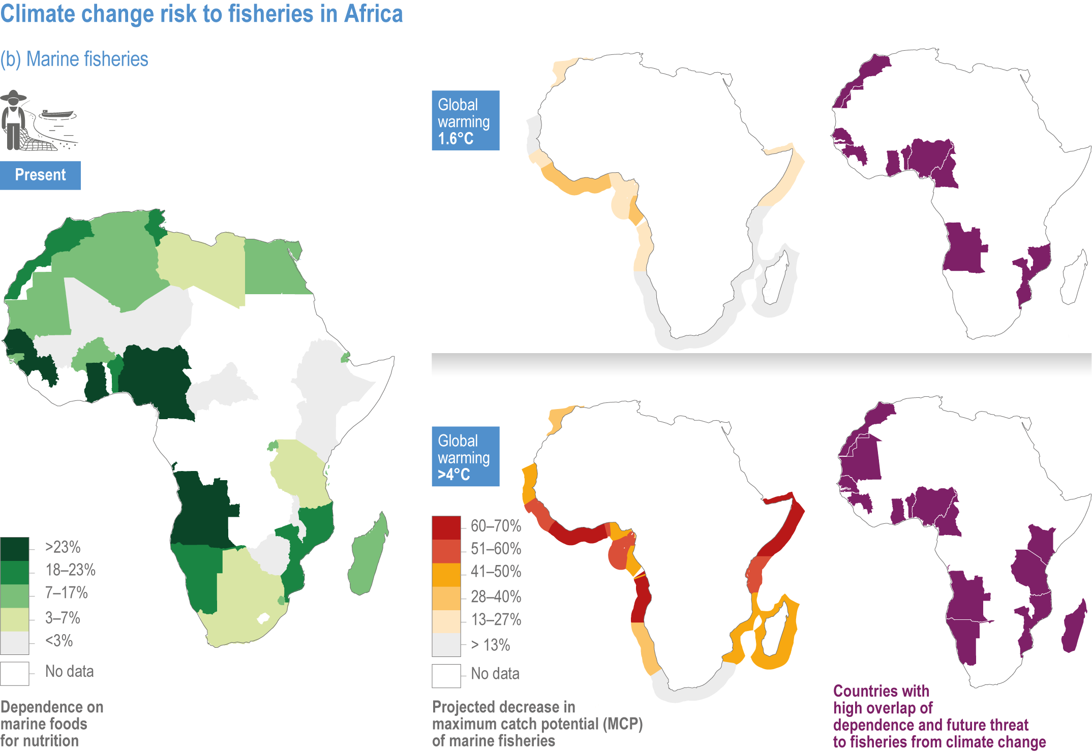
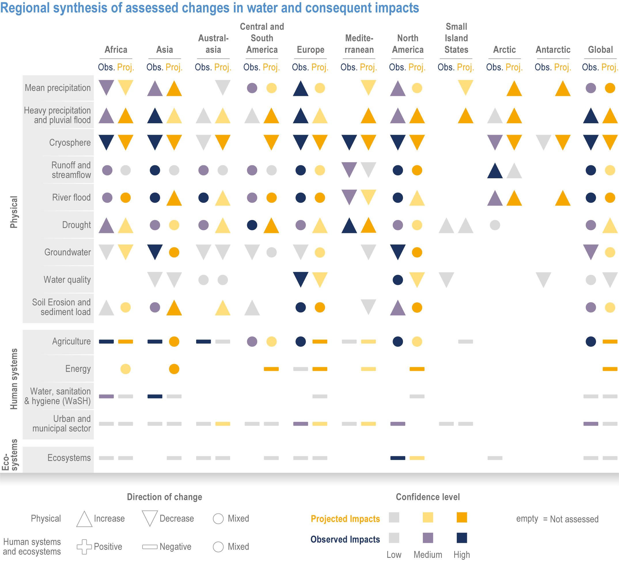
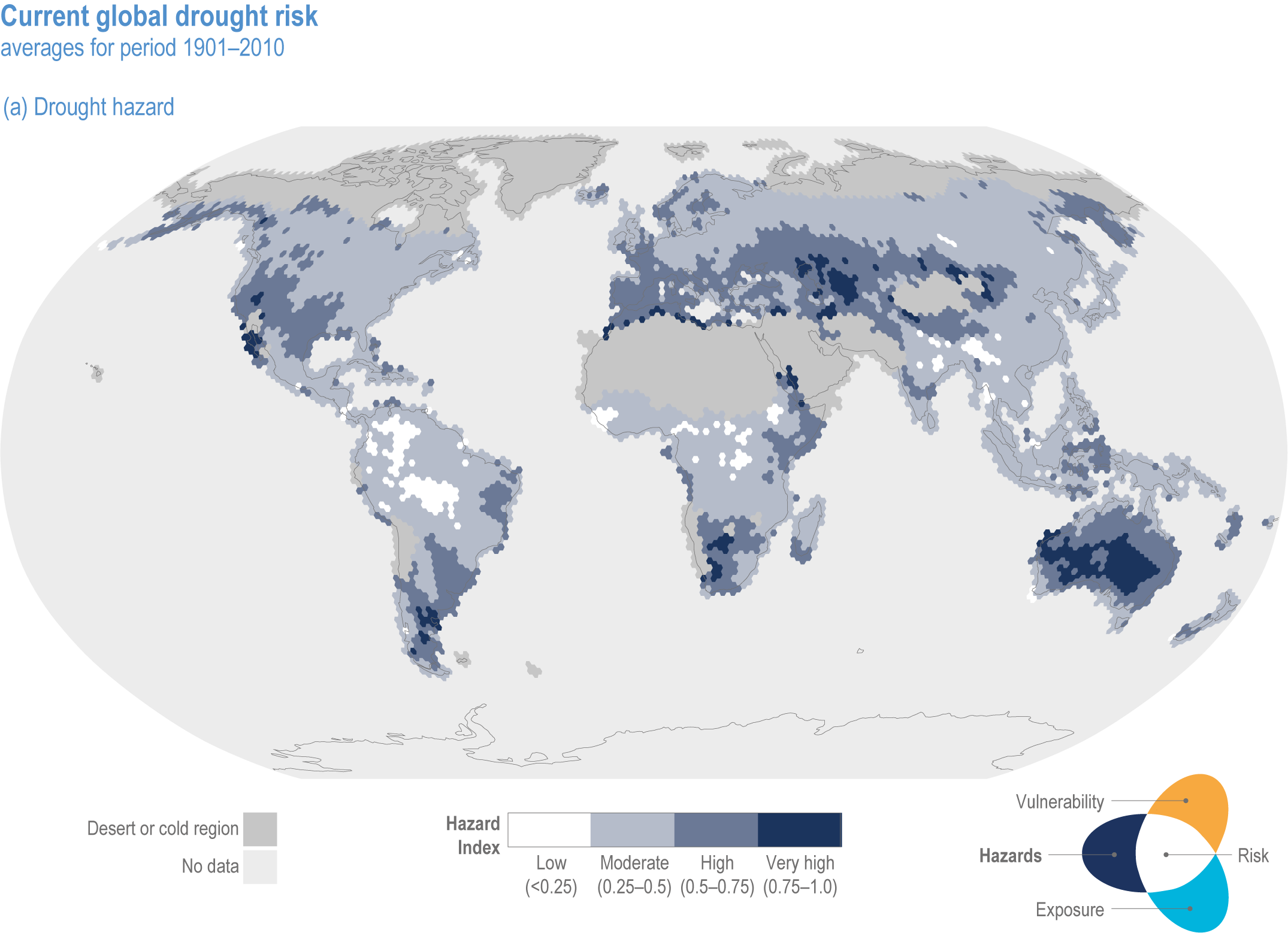
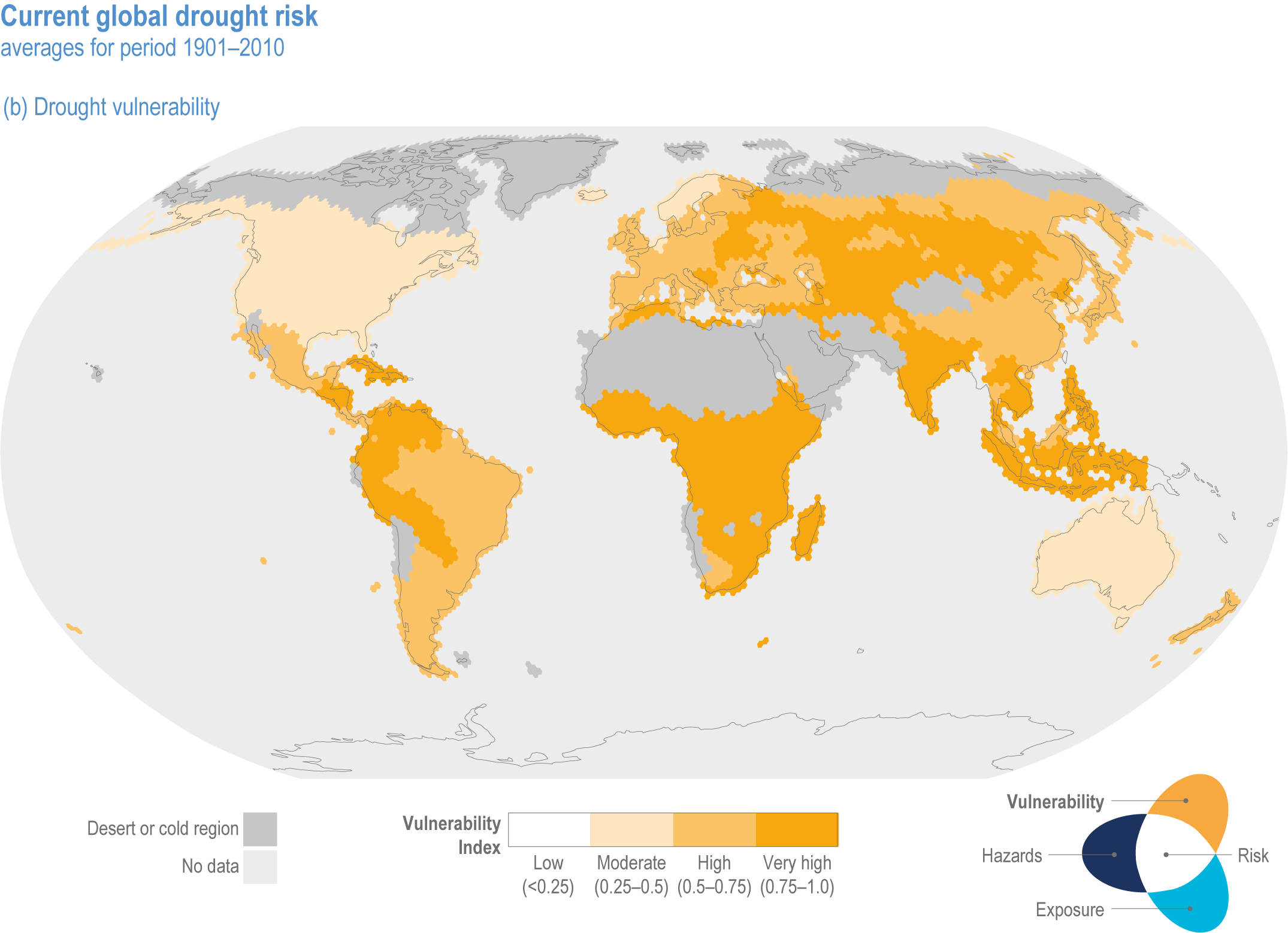
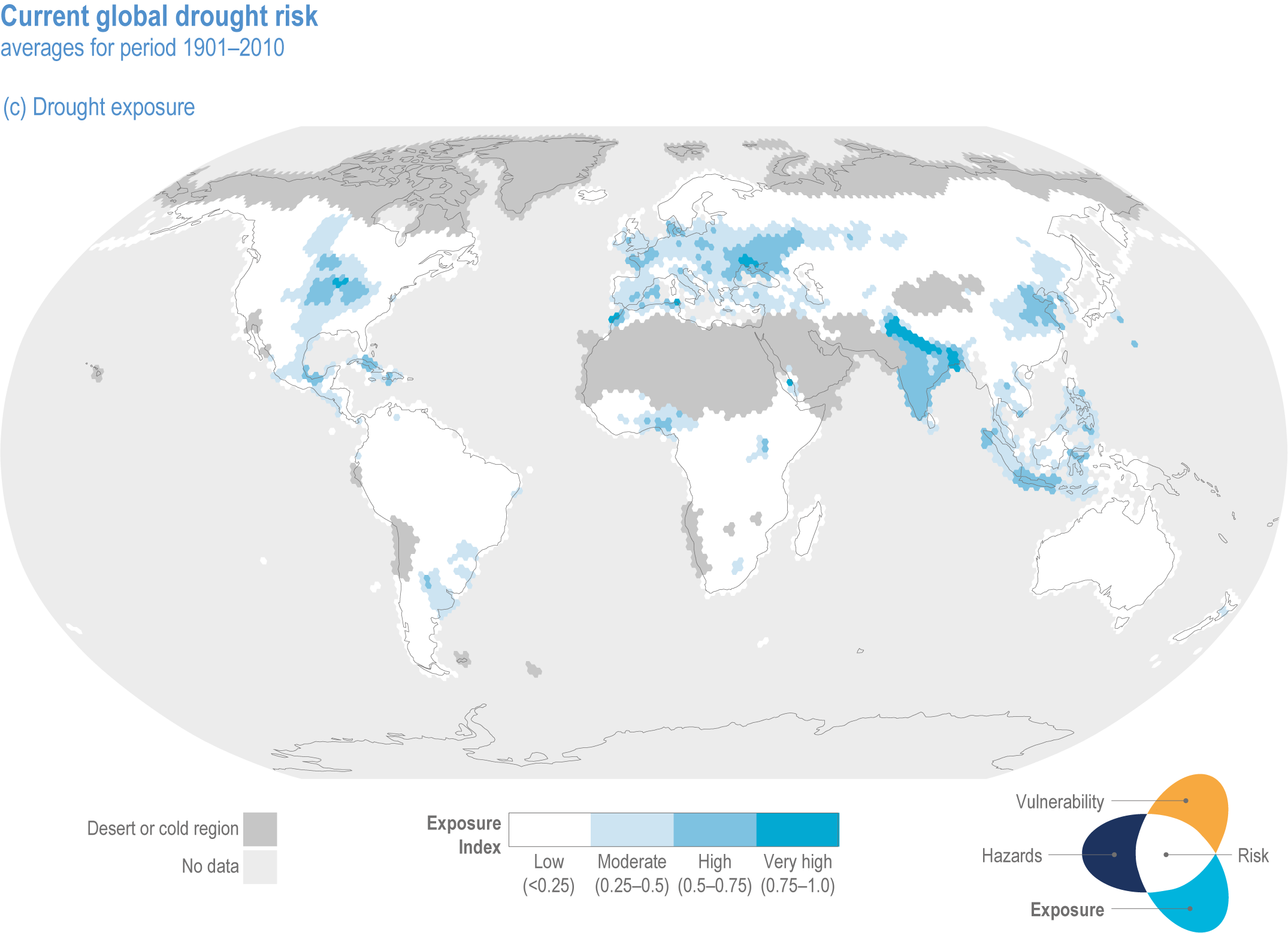
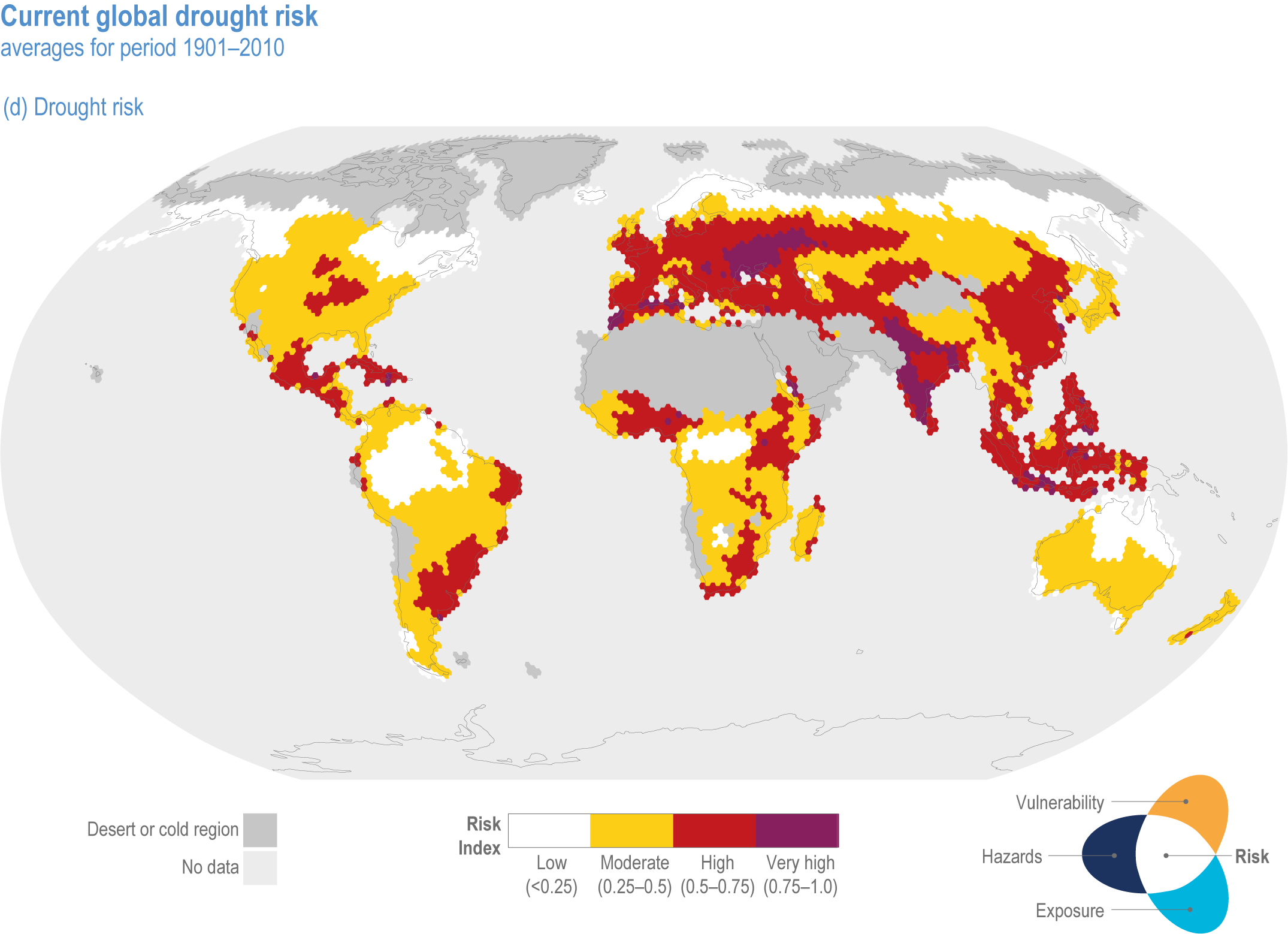
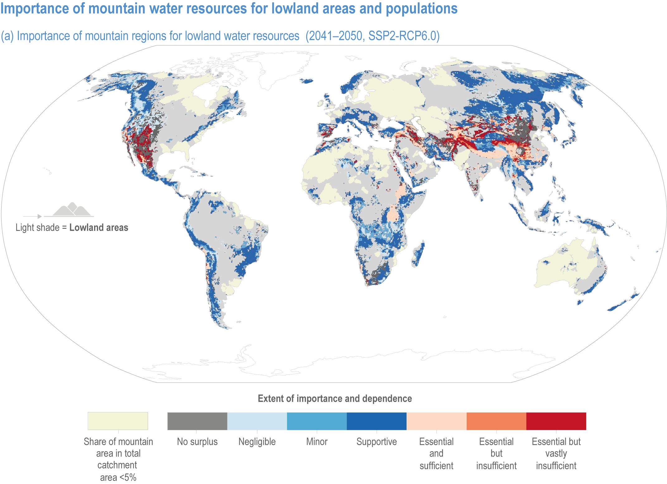
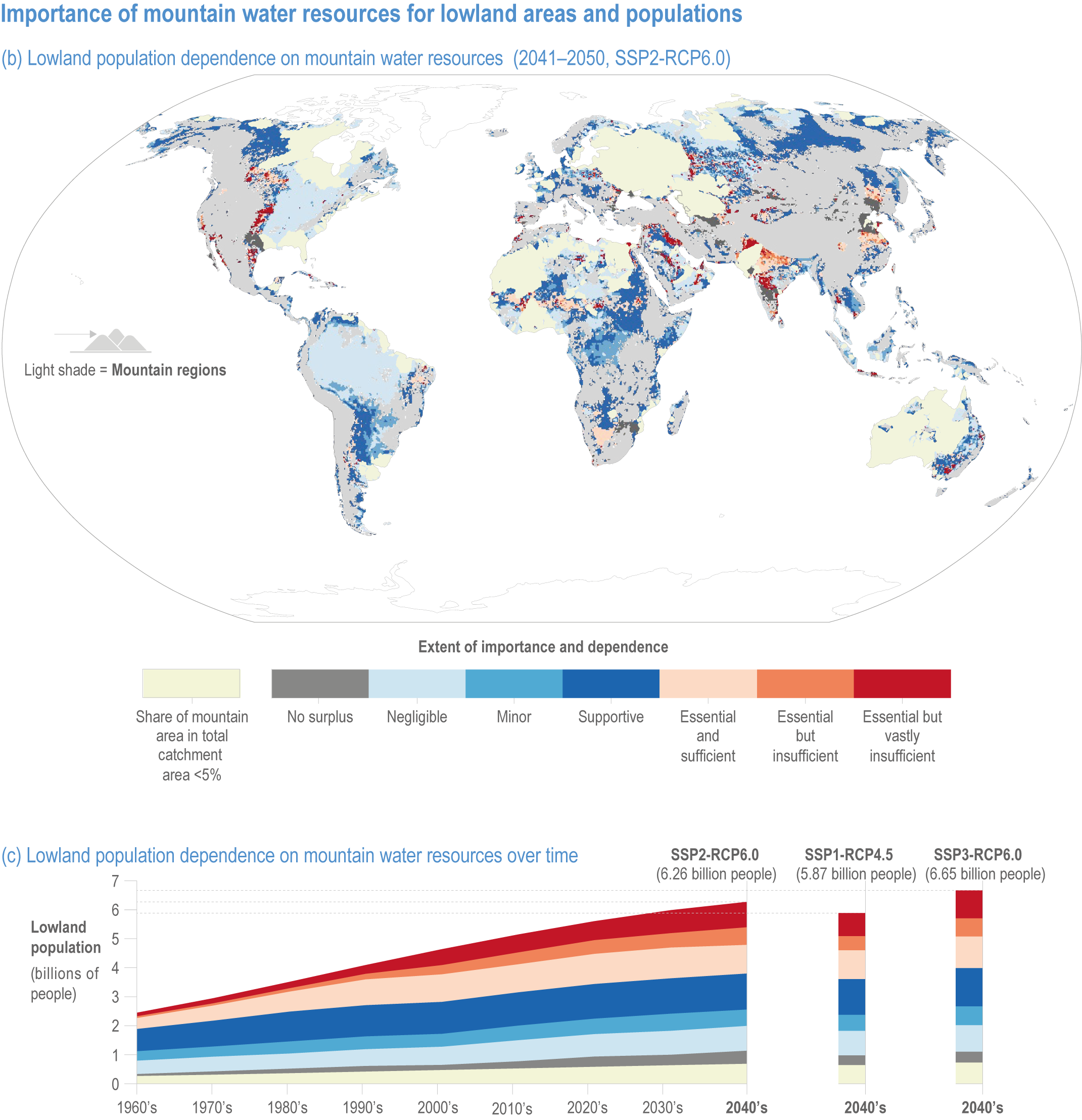
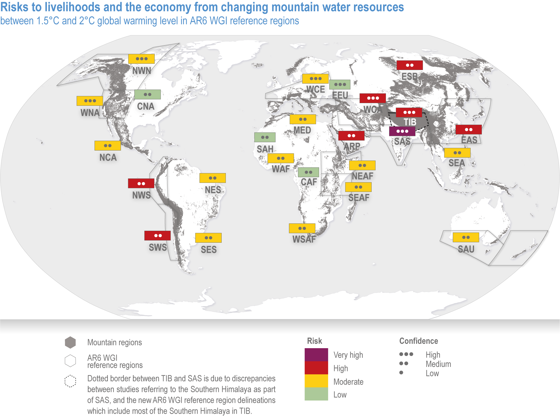
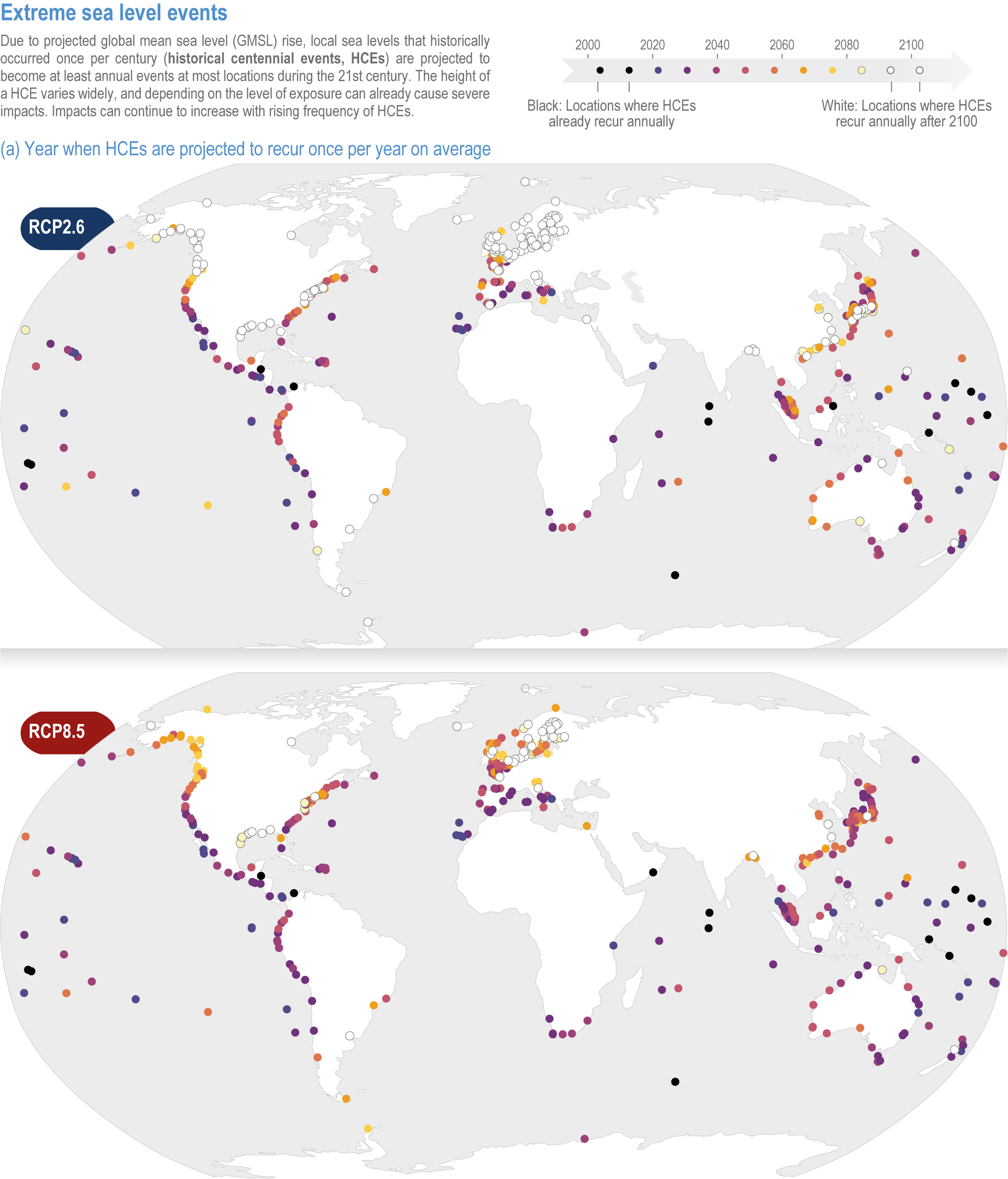
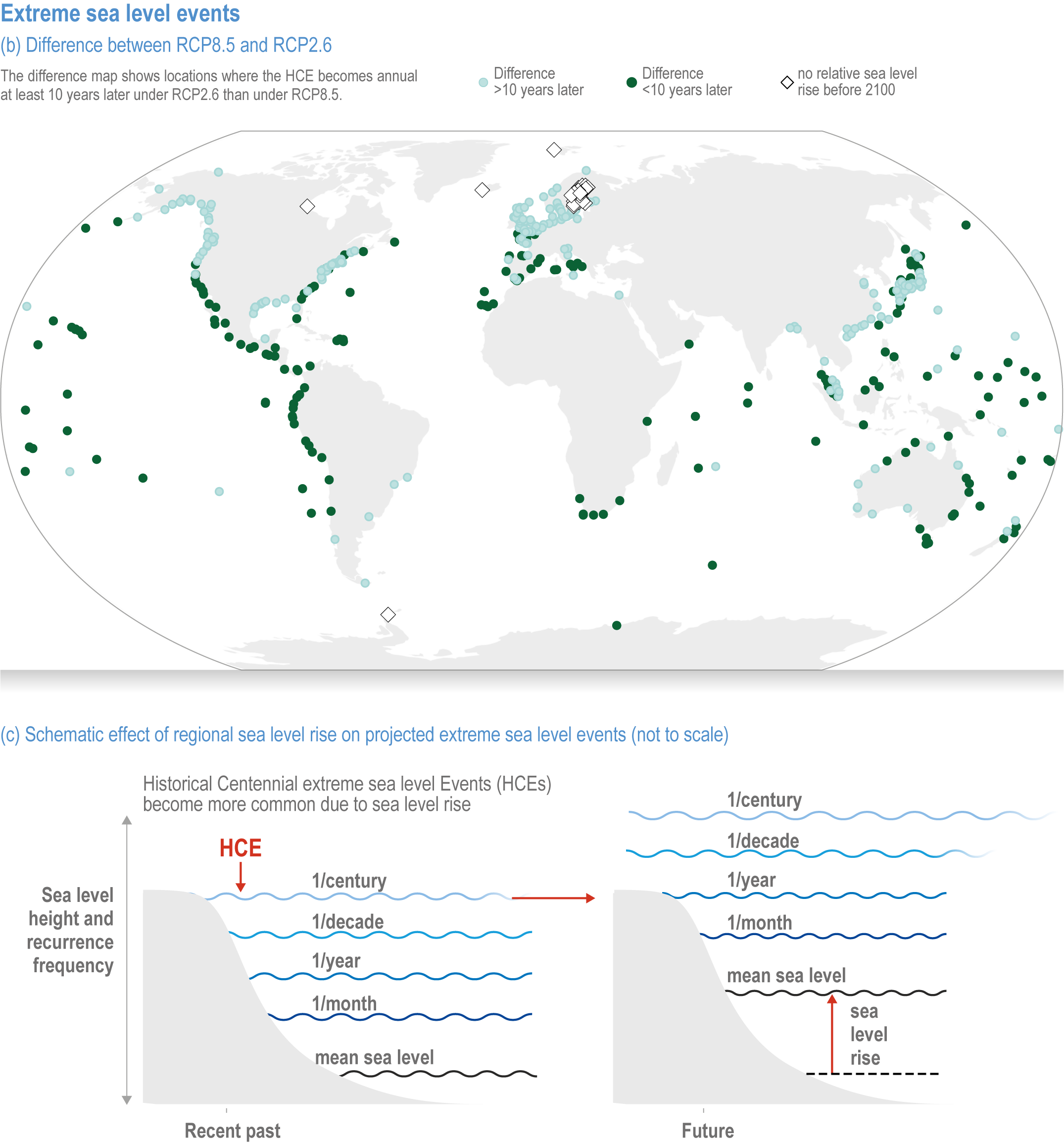
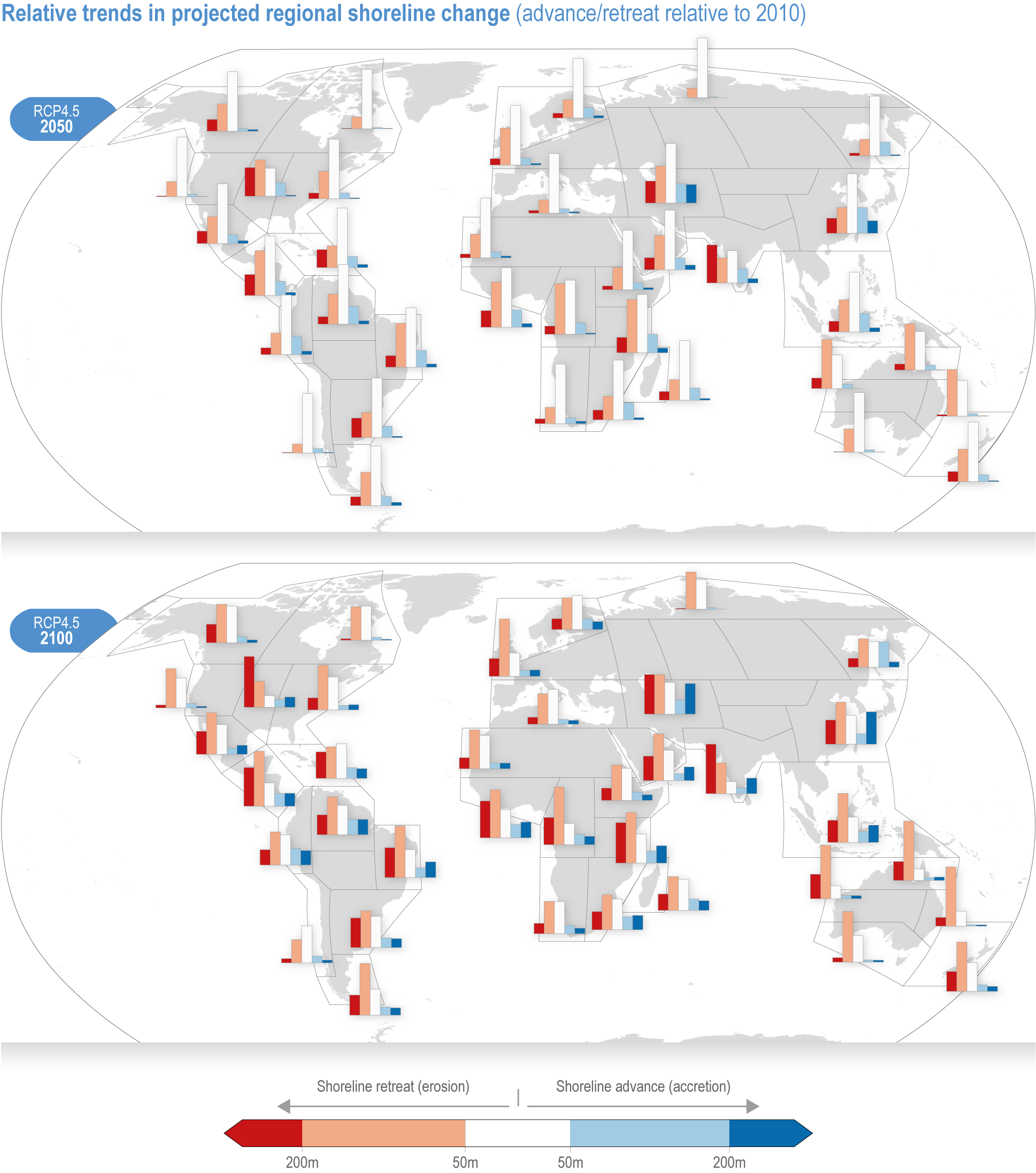
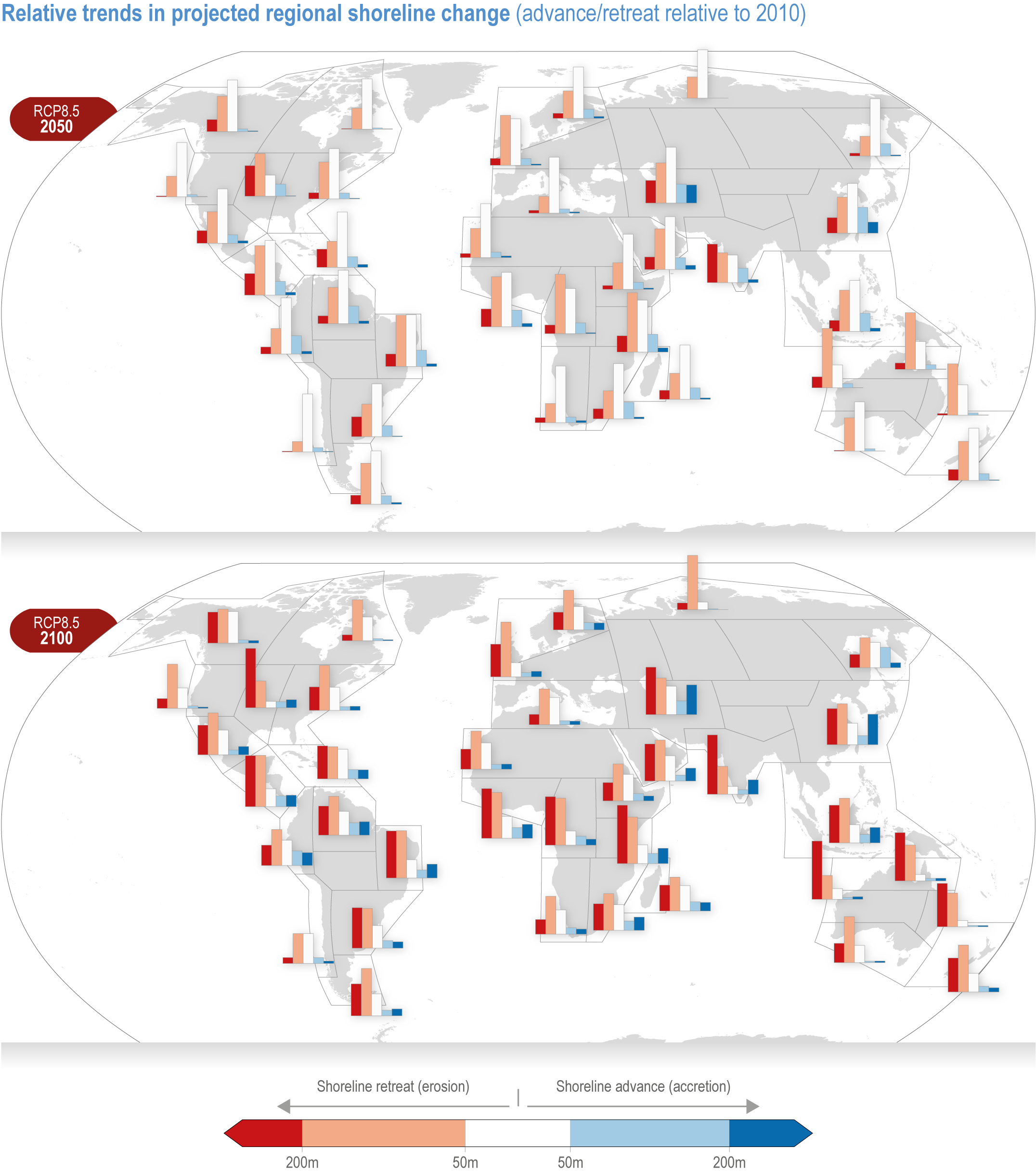
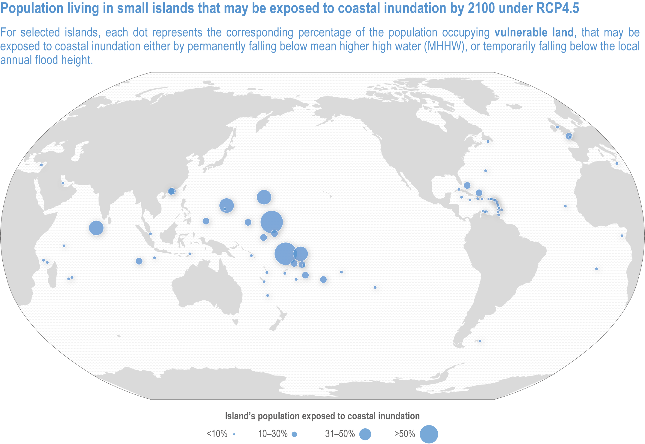
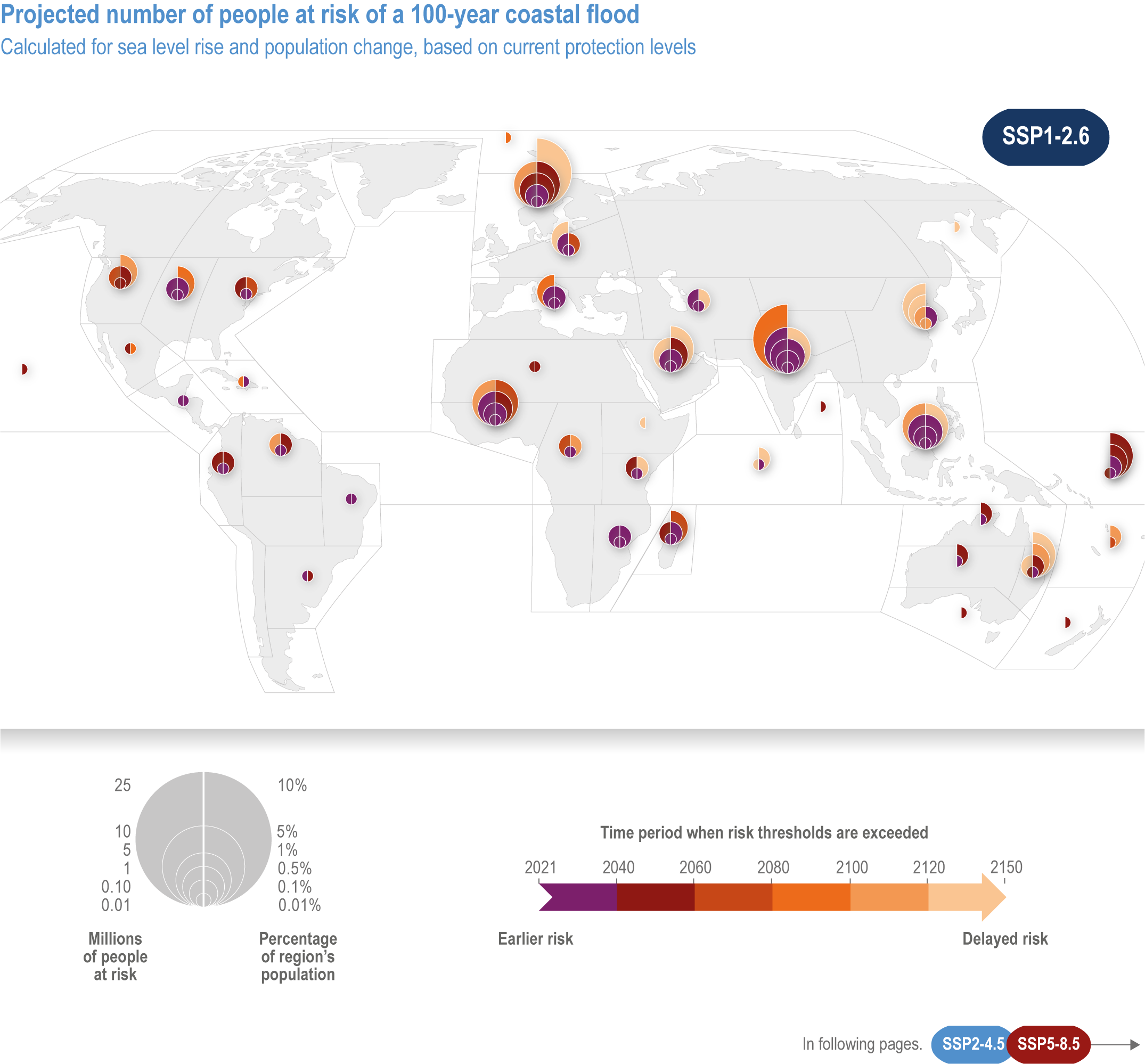
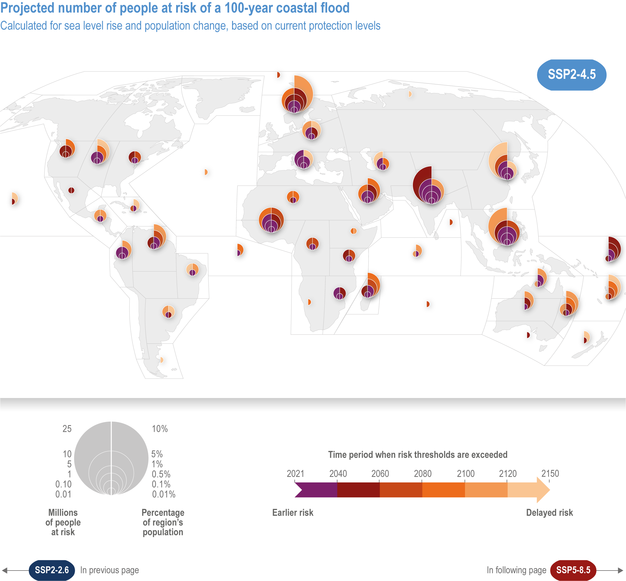
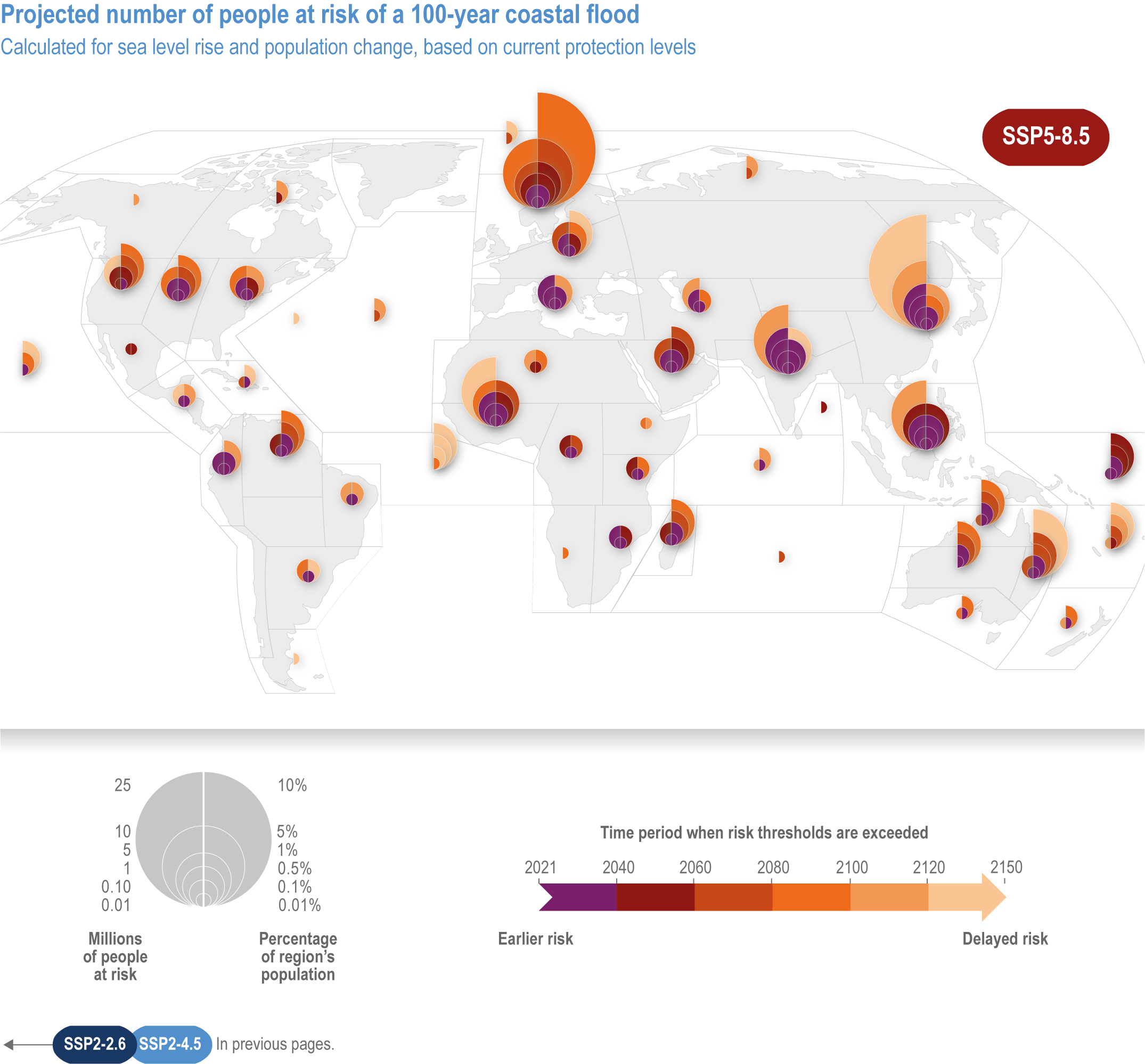
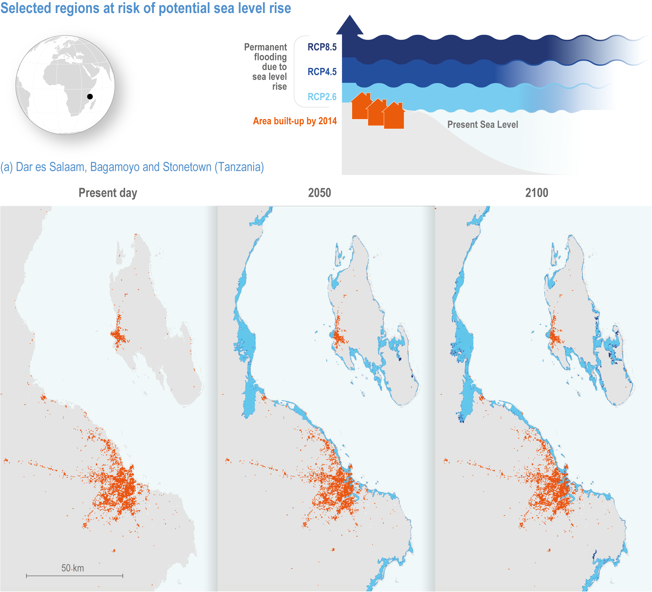
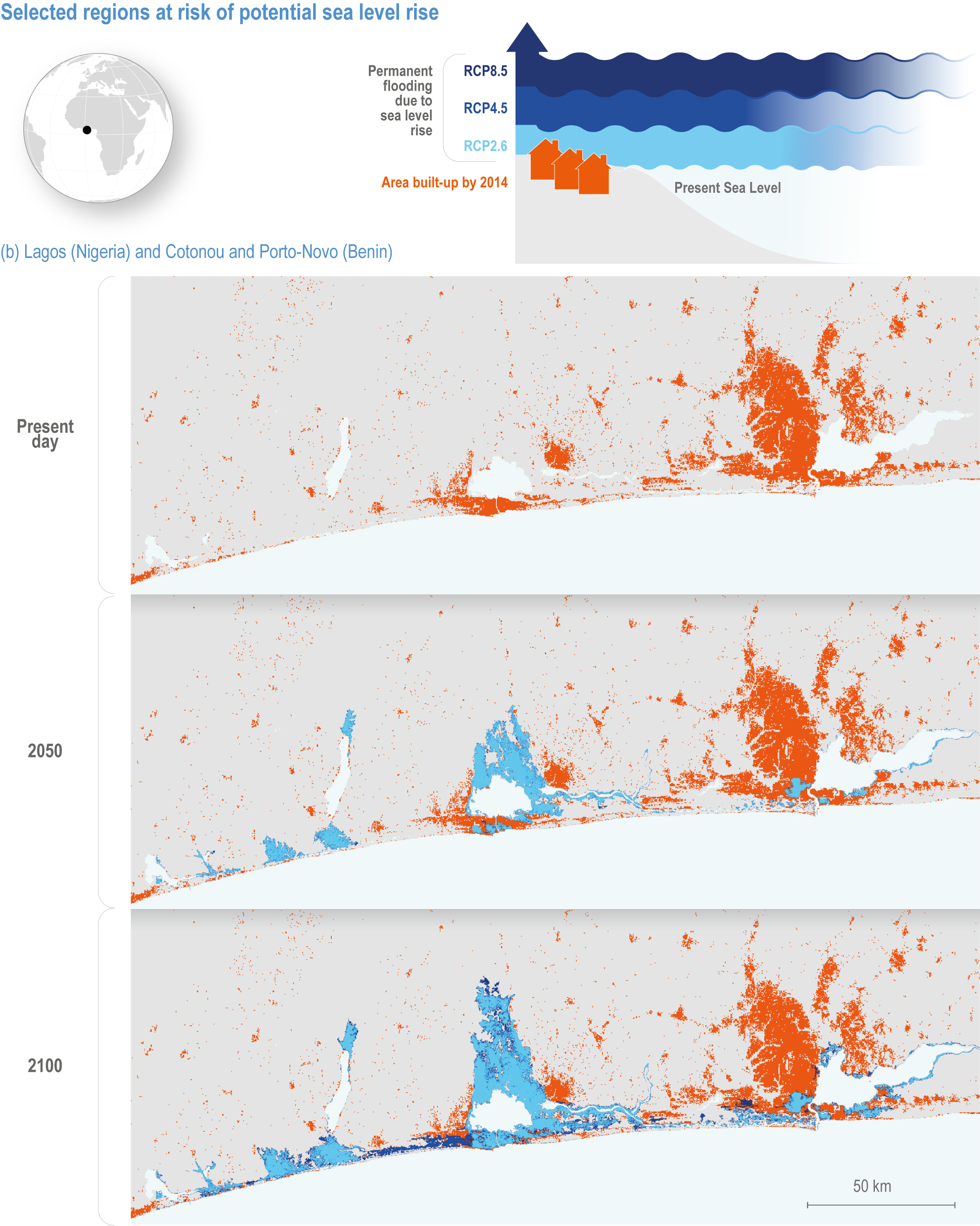
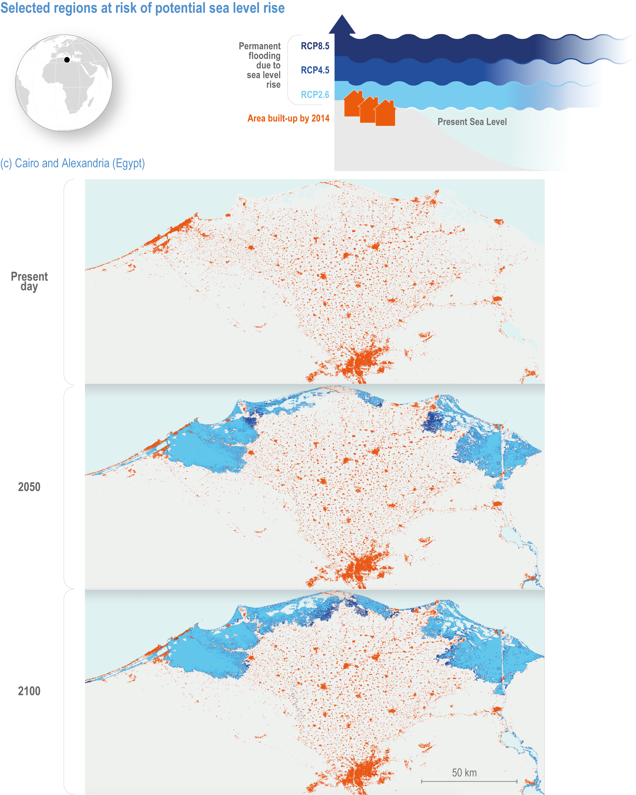
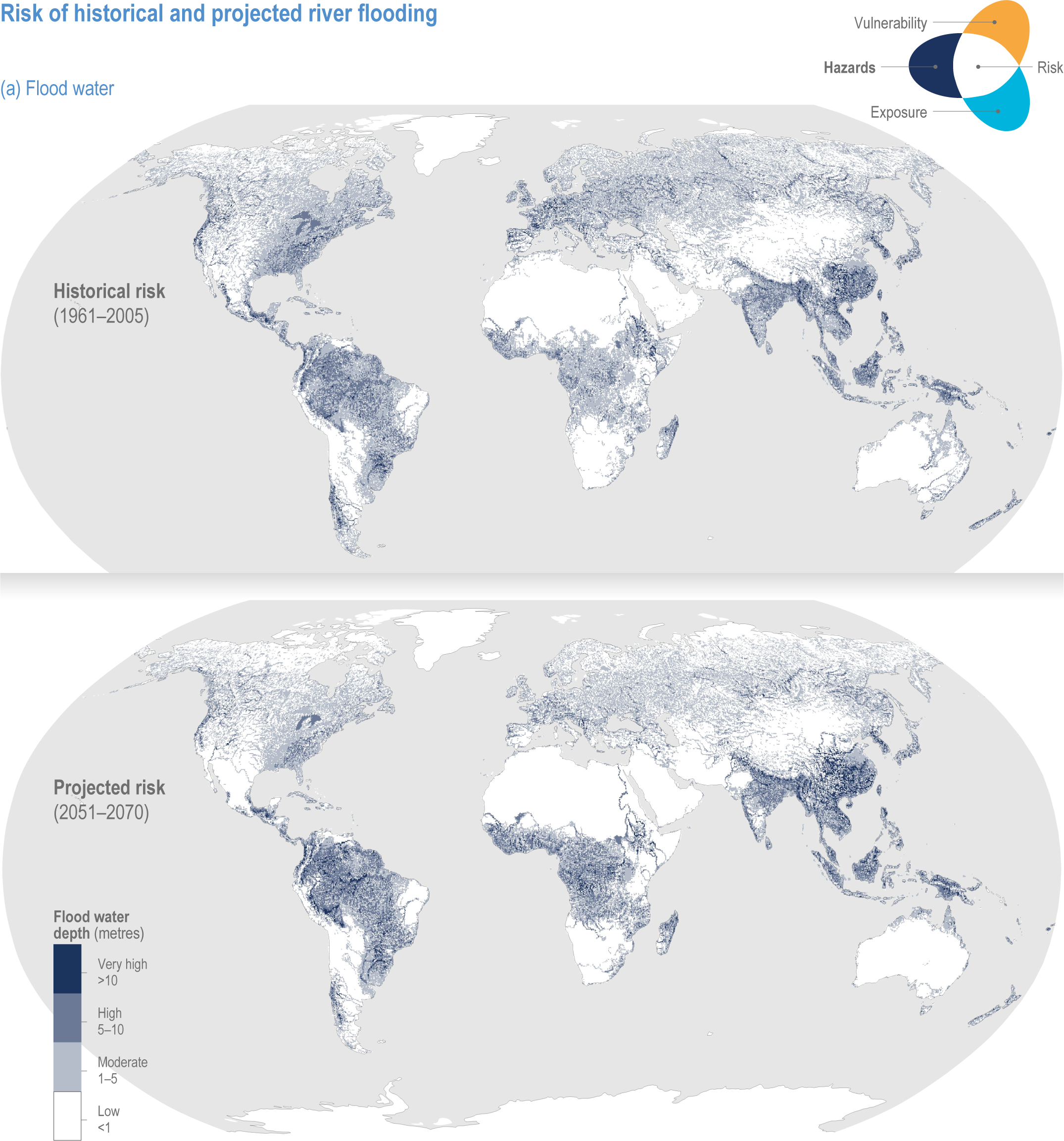
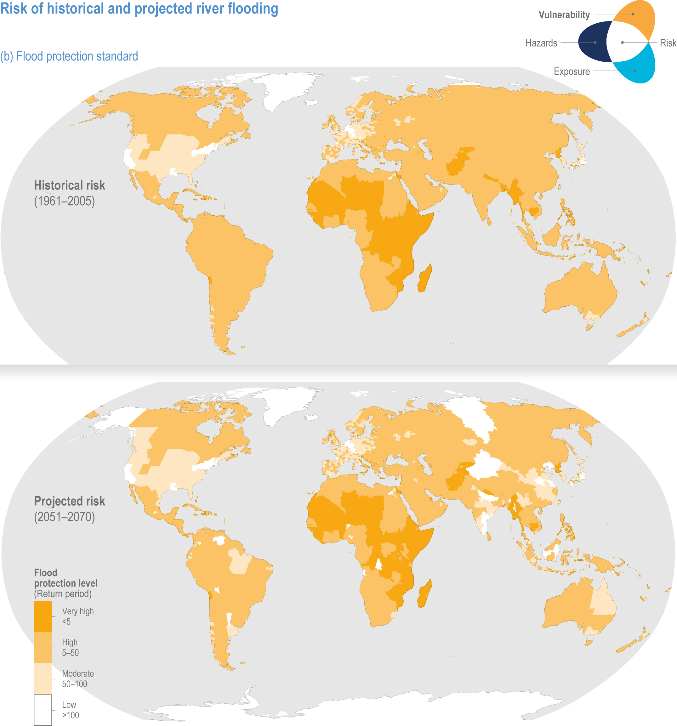
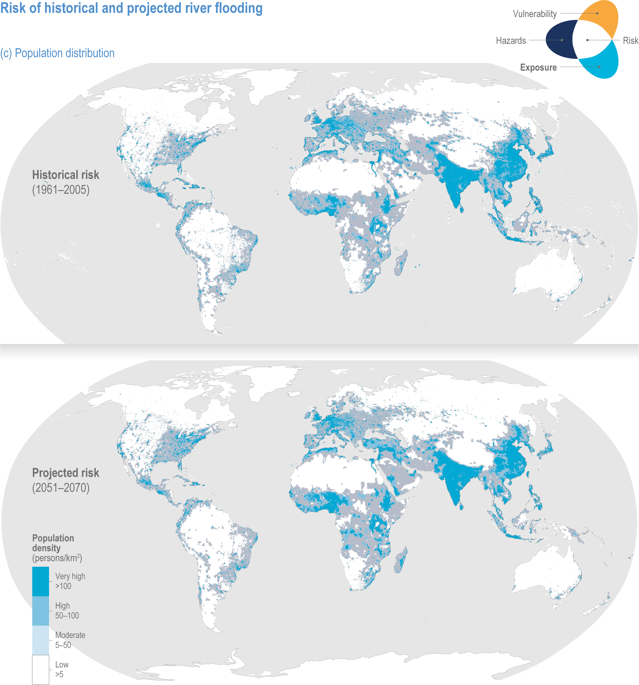
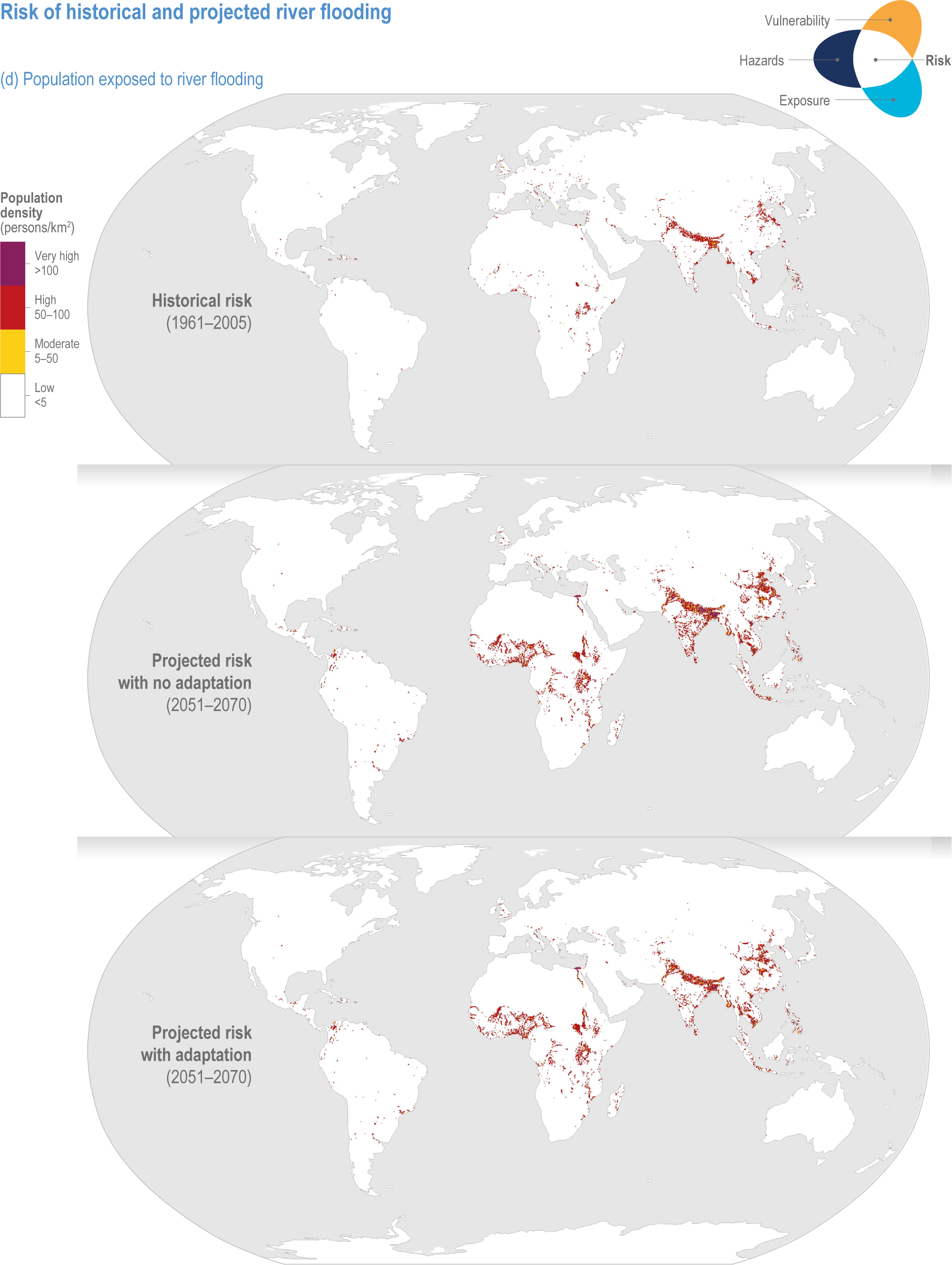 Figure AI.44d | Risk of historical and projected river flooding.
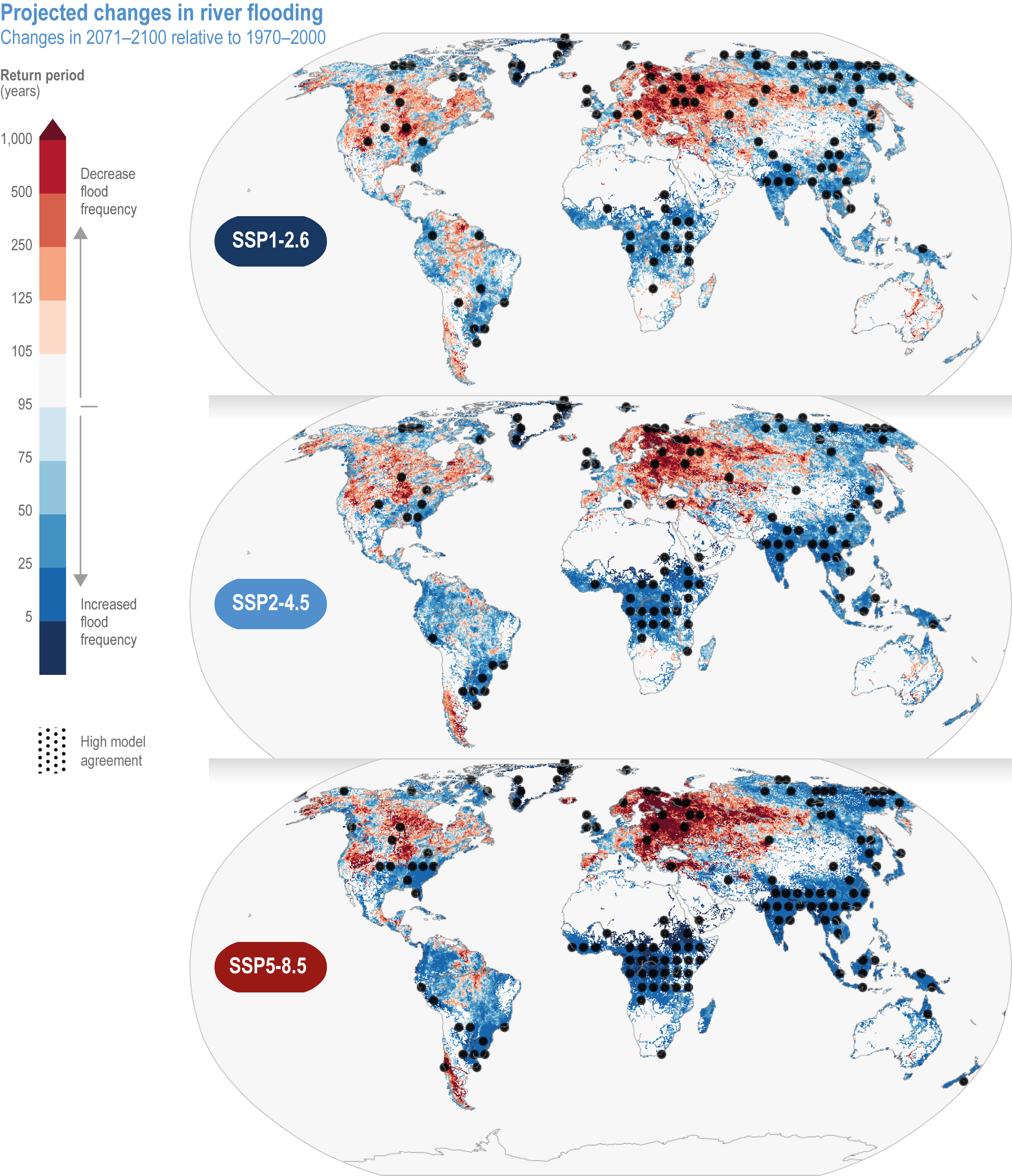
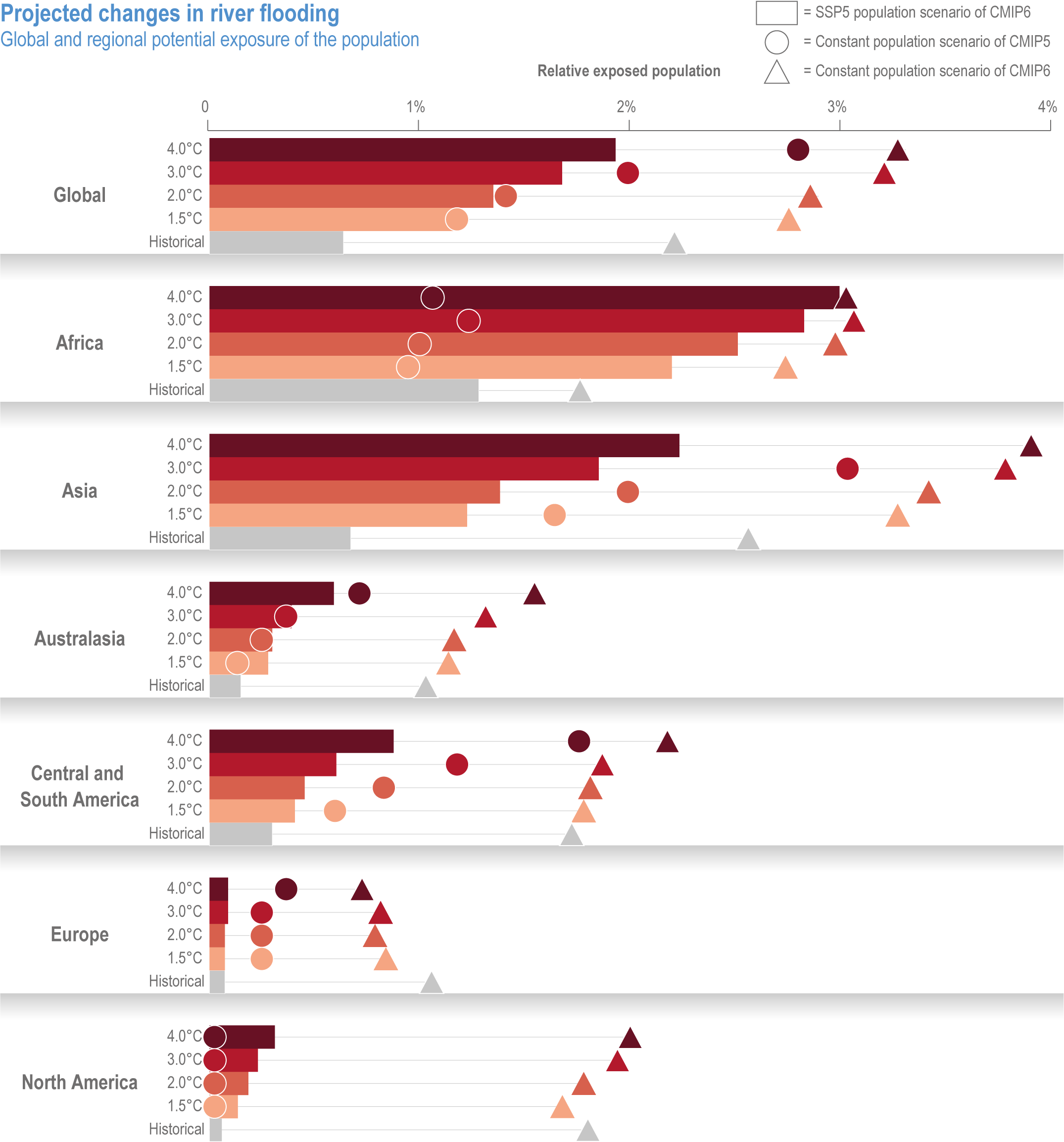
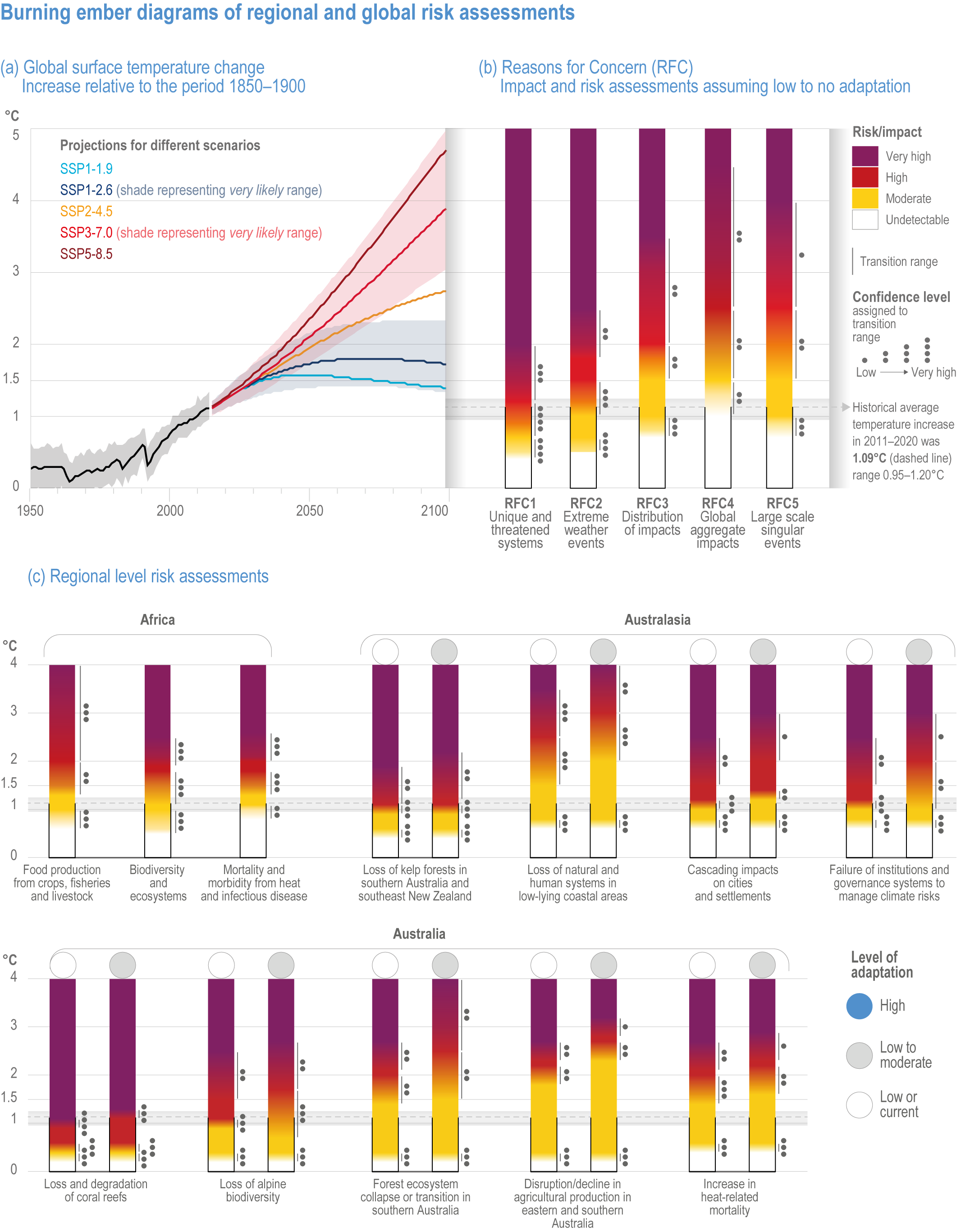
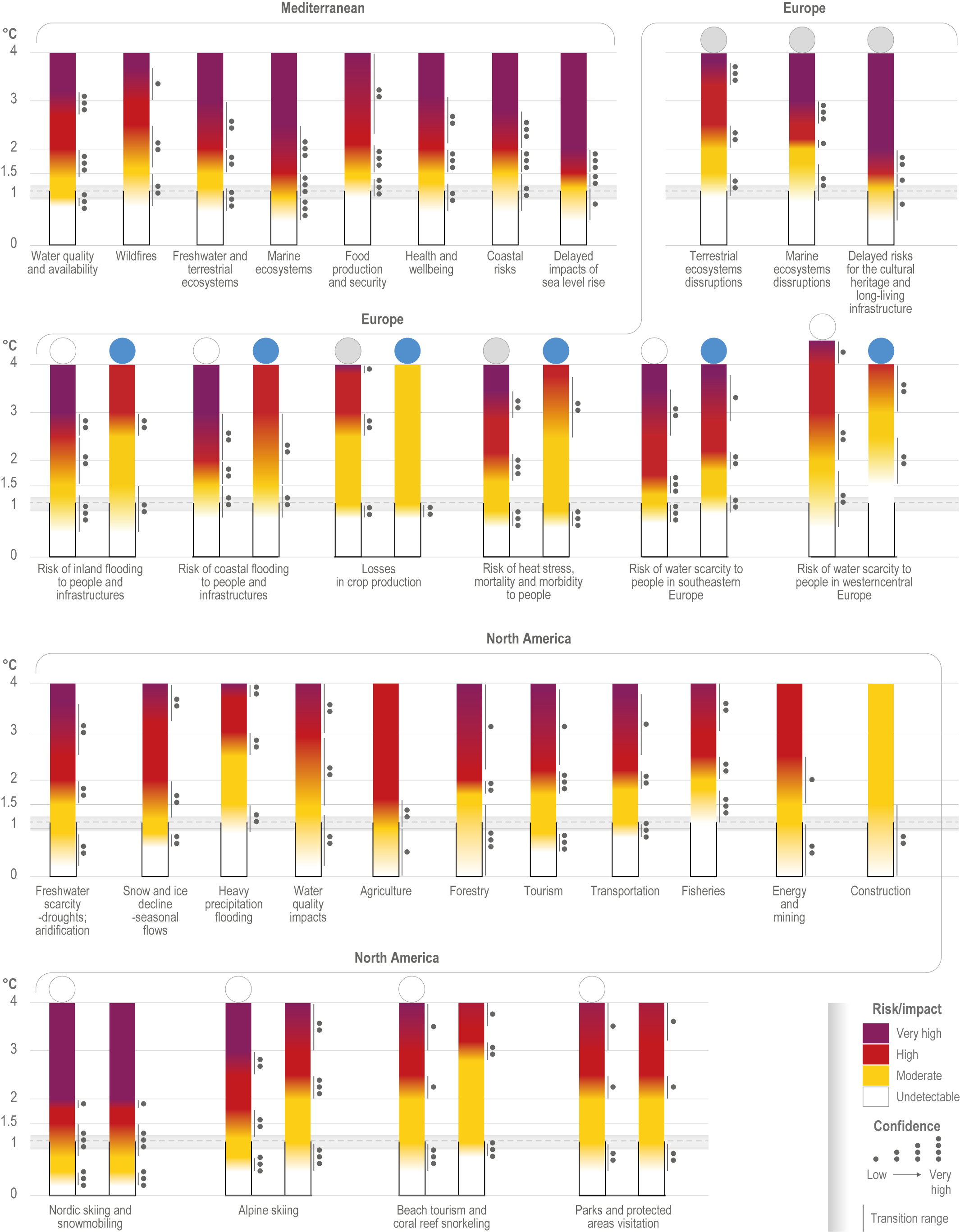
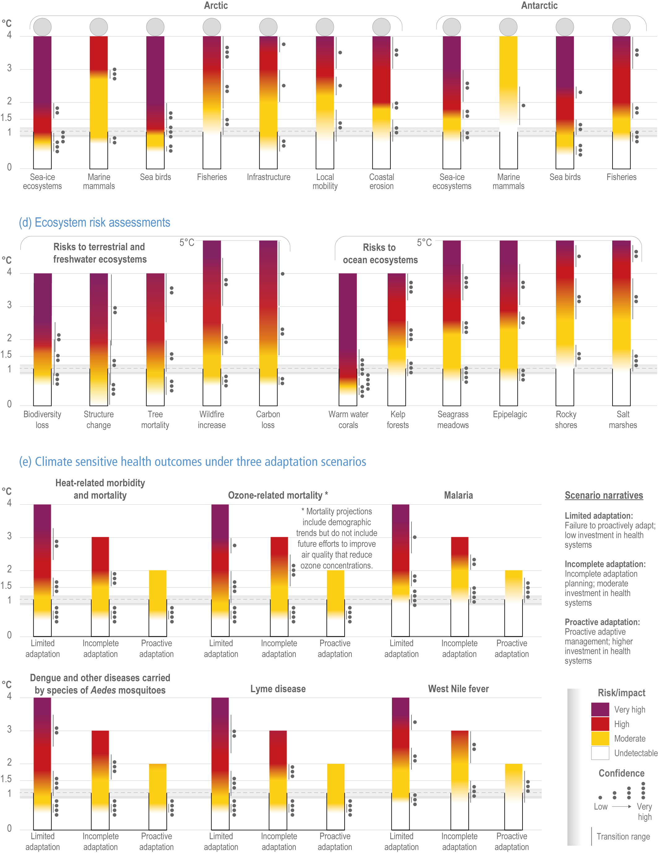
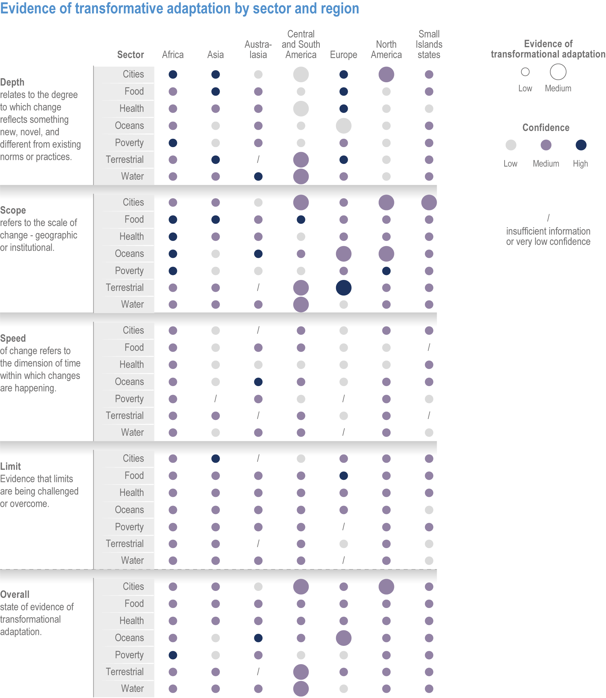
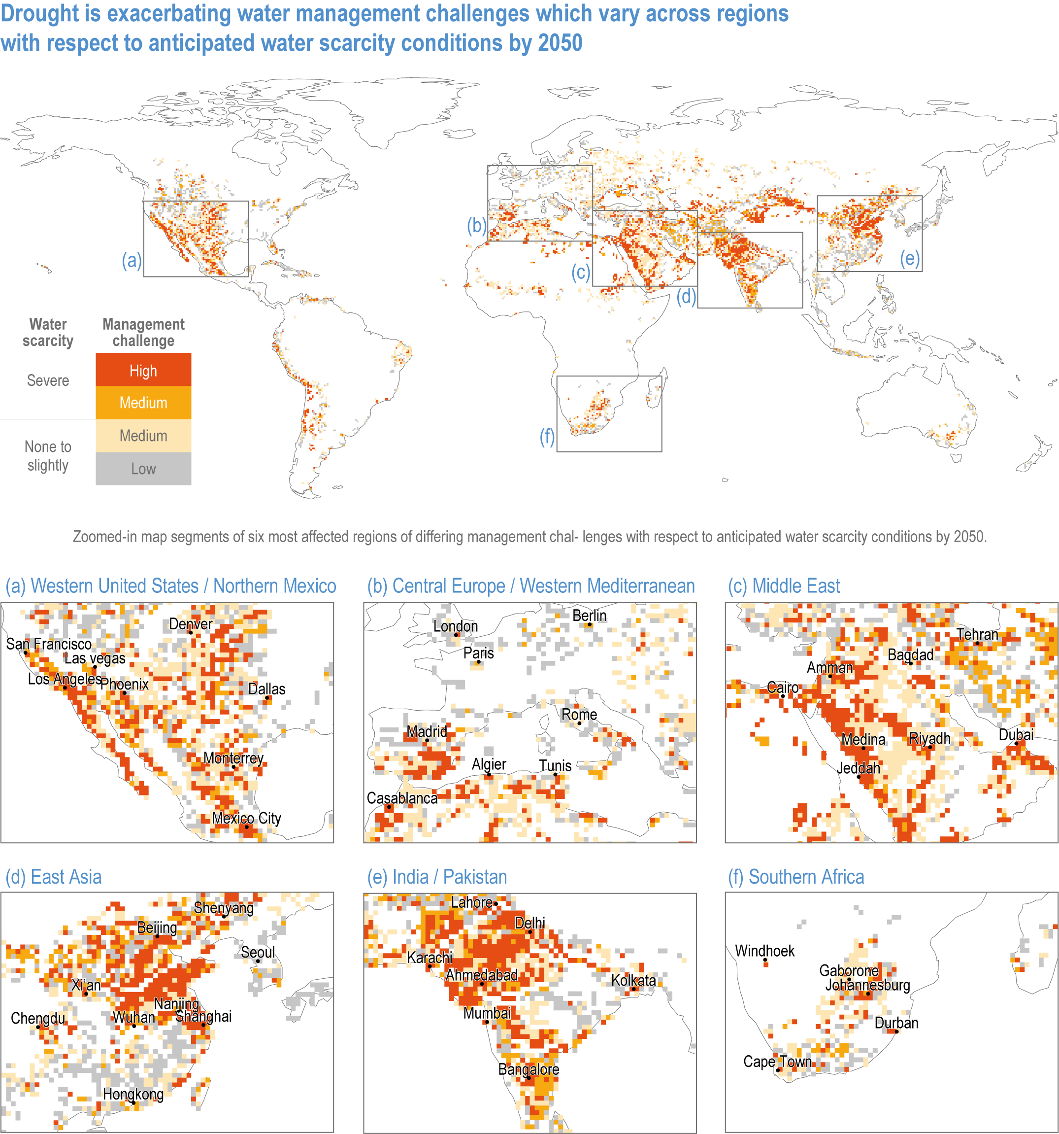
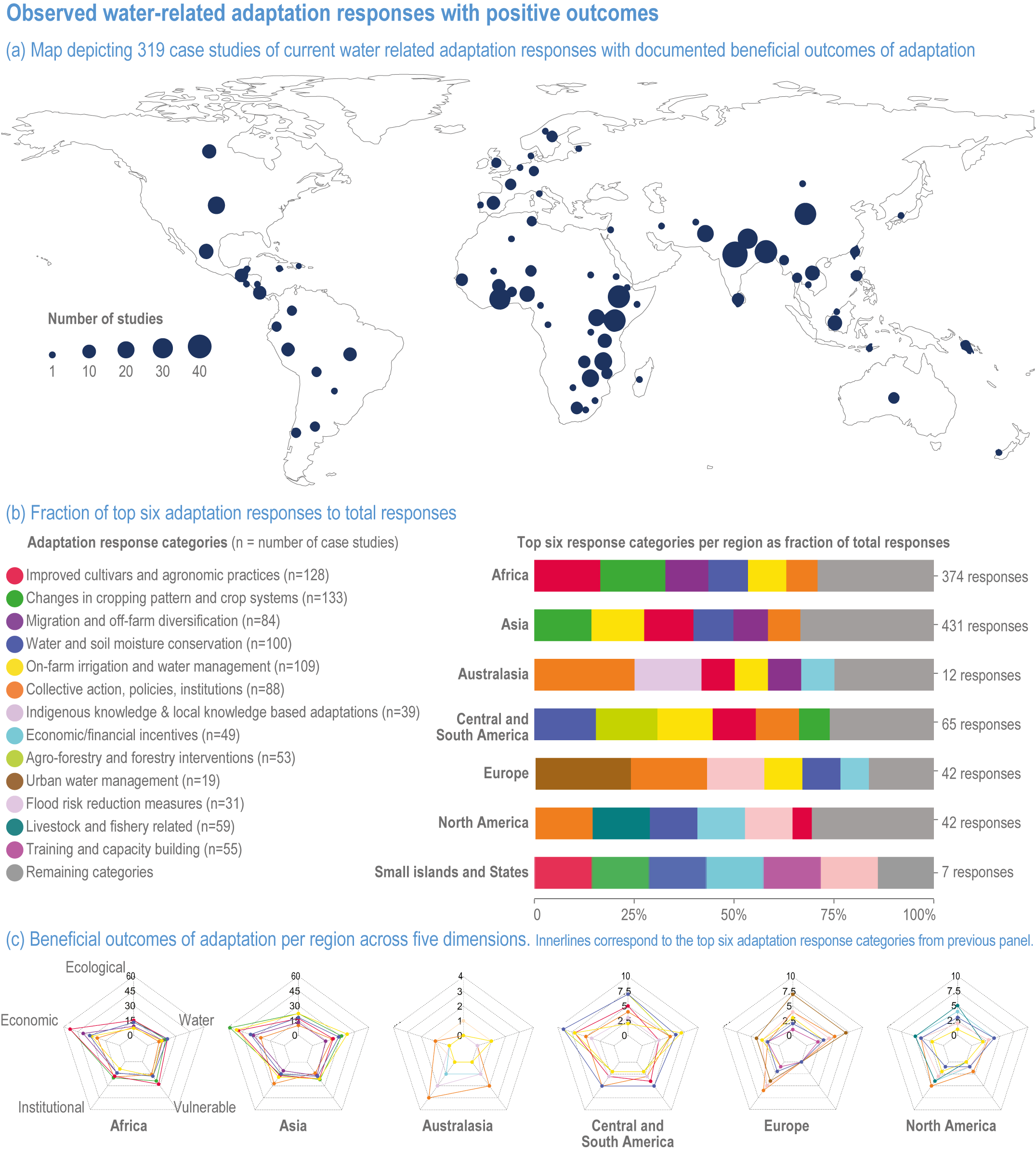
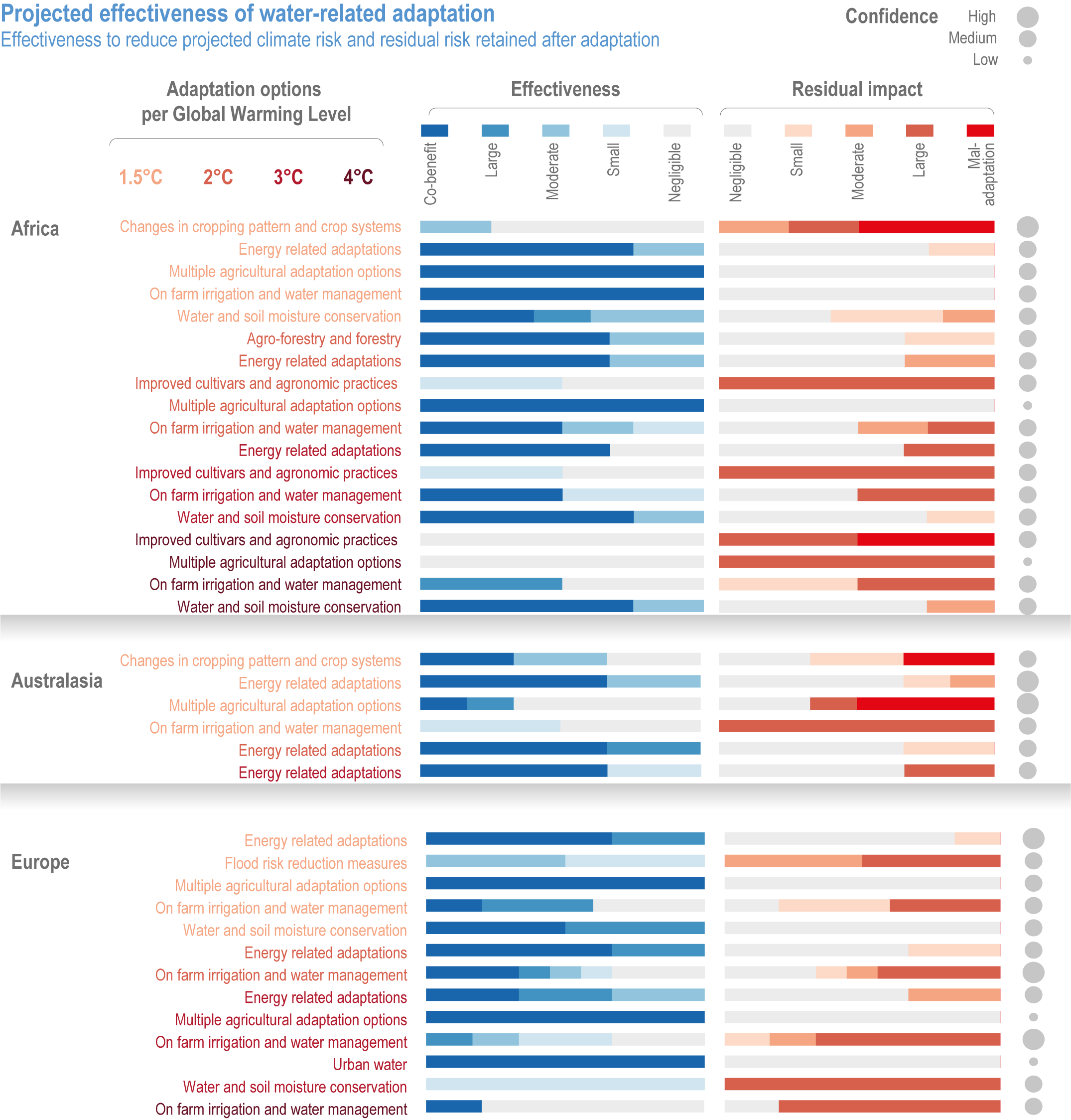
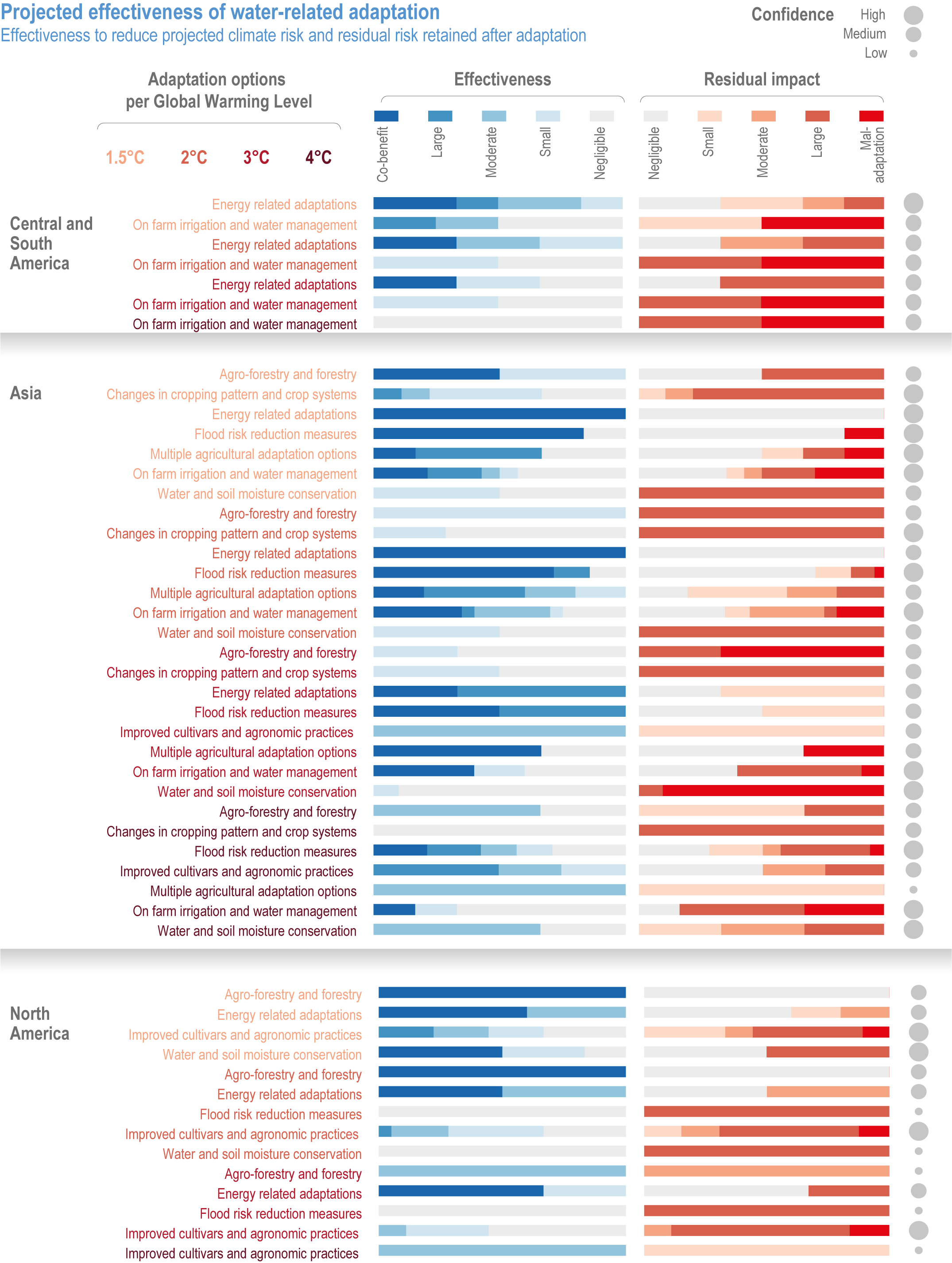 Figure AI.50b | Projected effectiveness of water-related adaptation options.
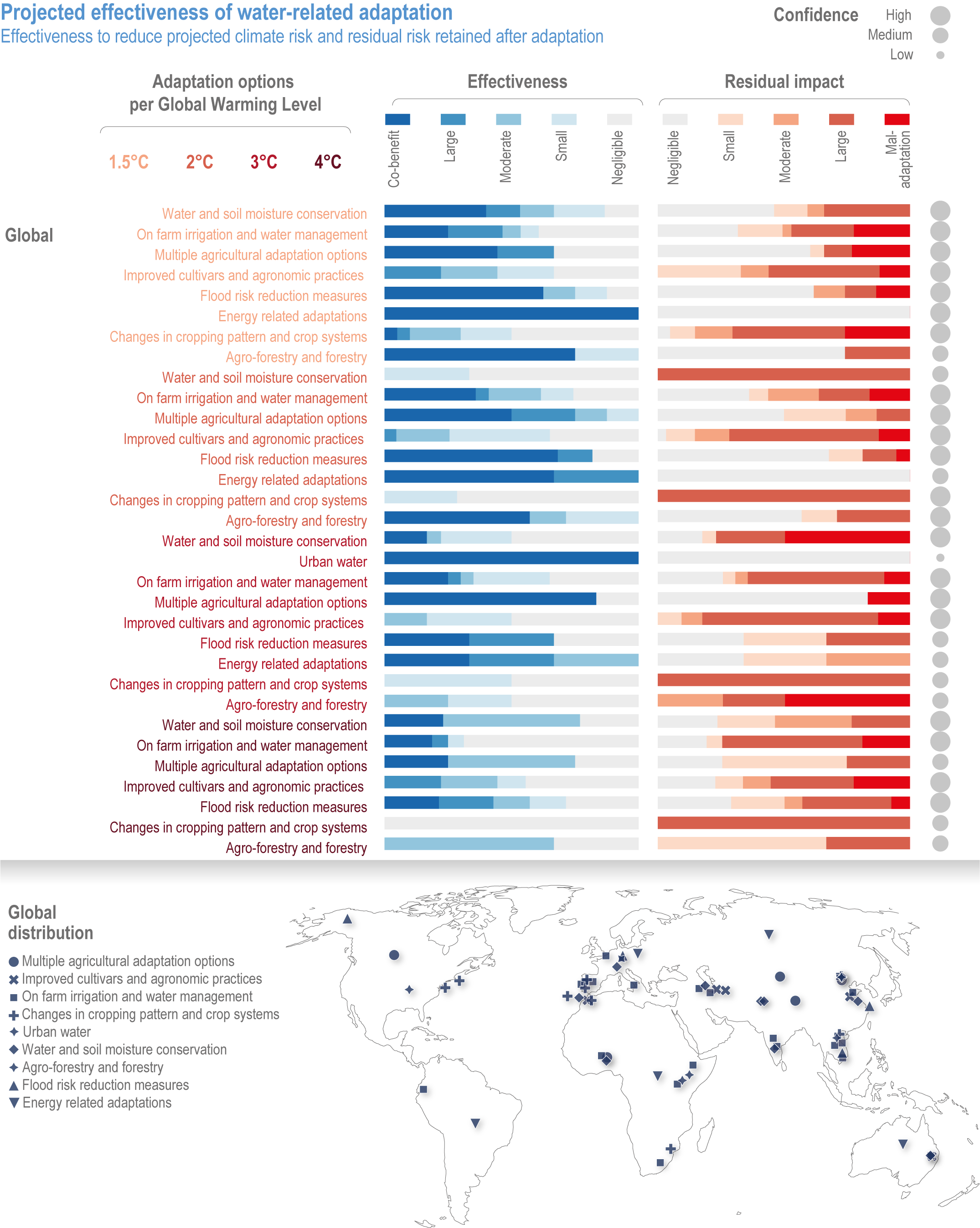
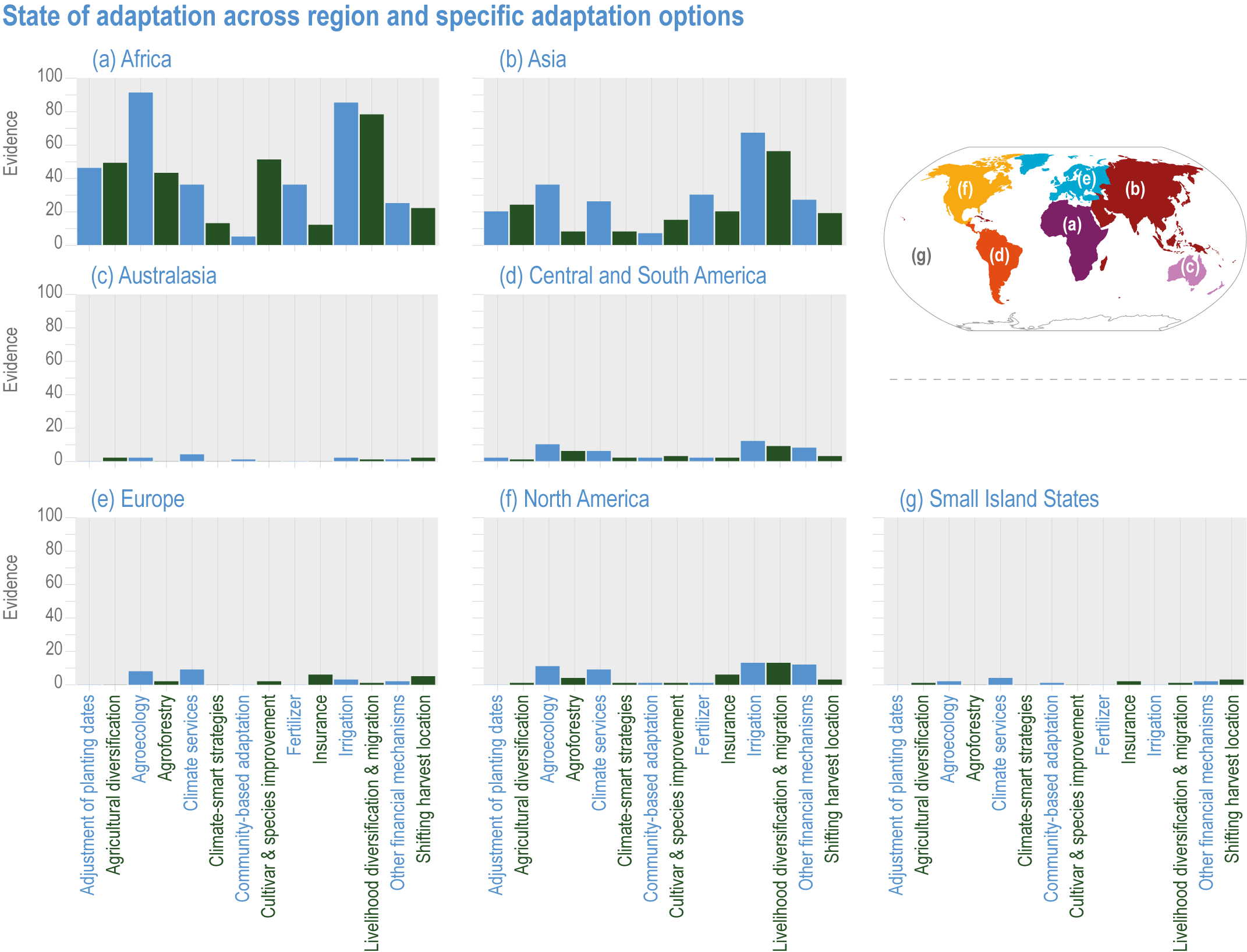
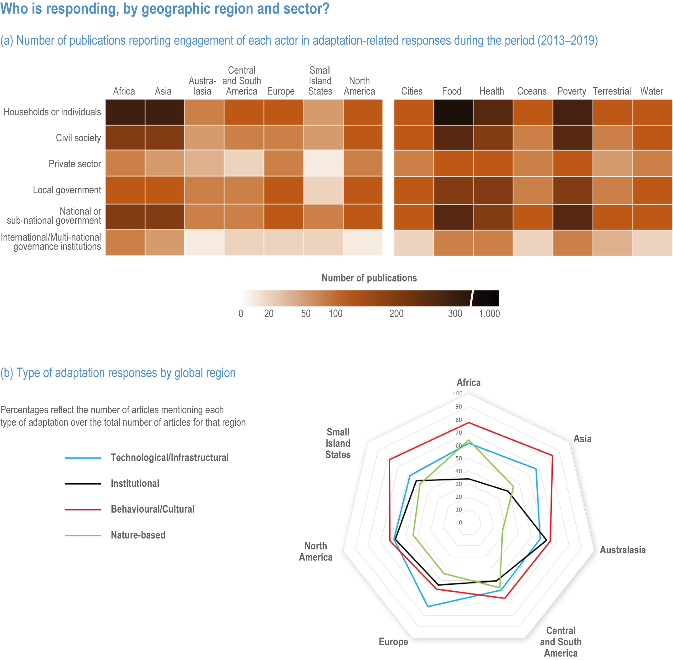
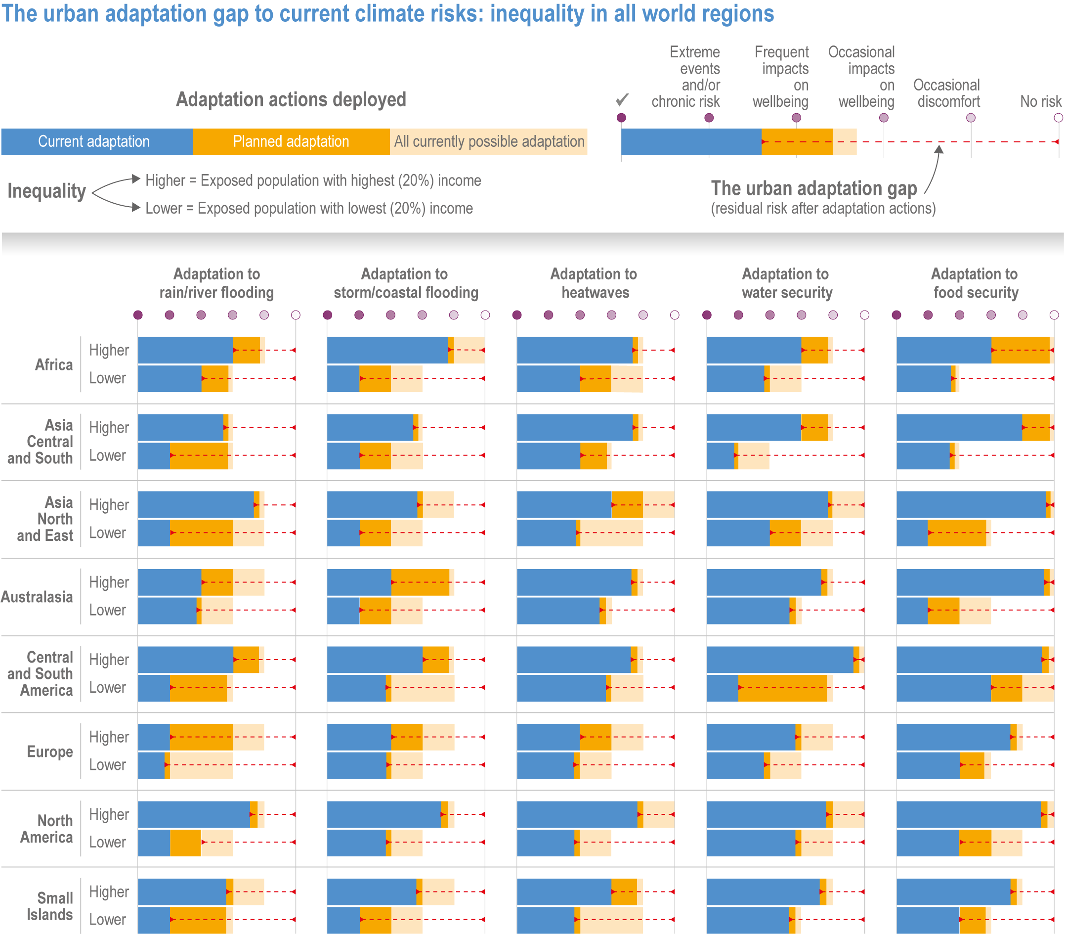
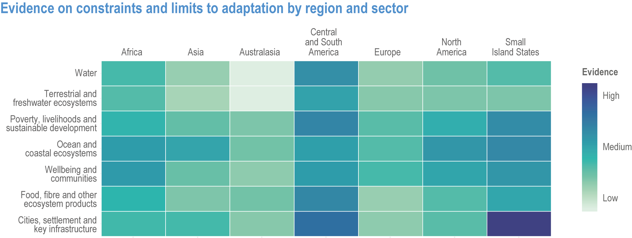
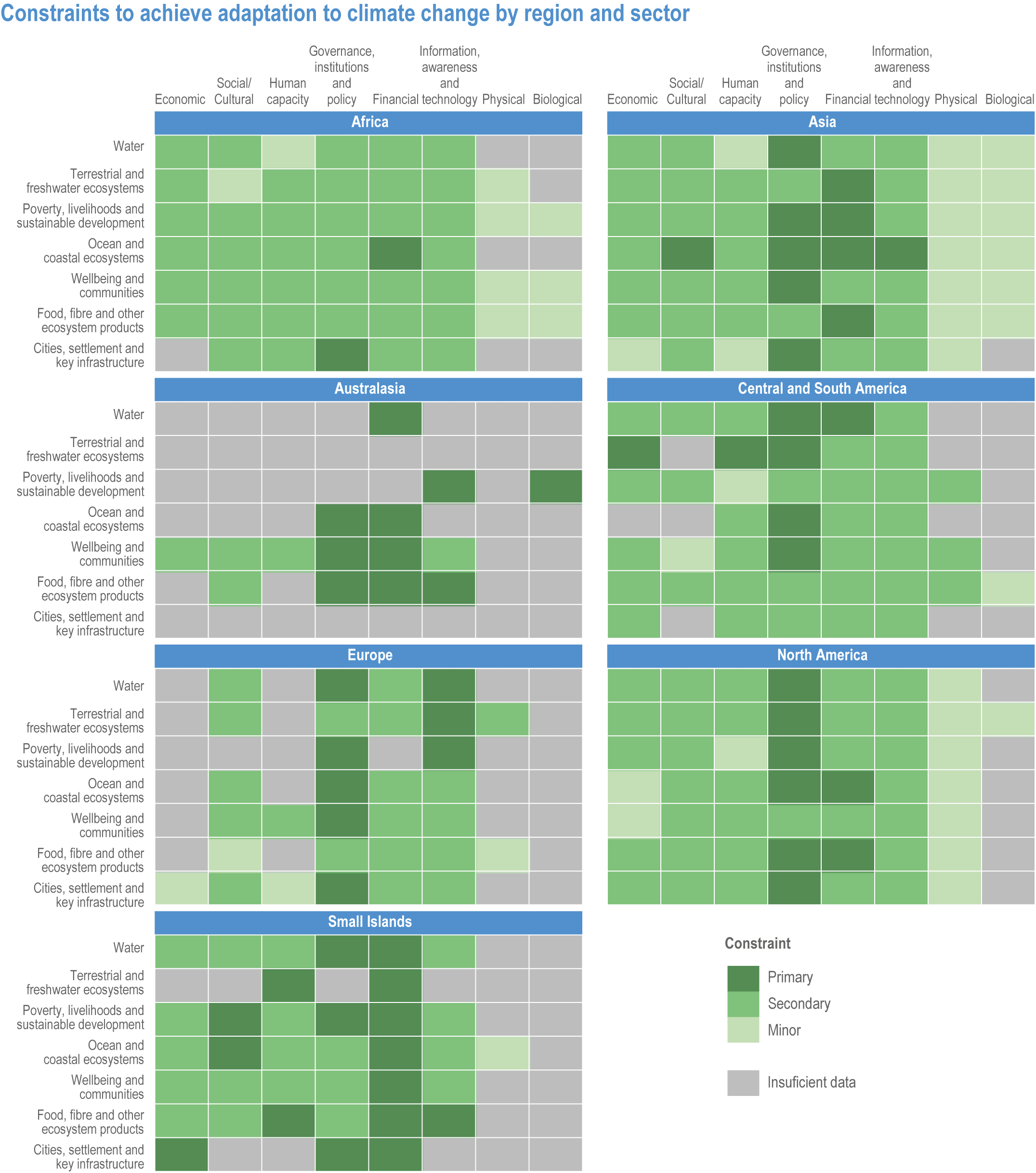
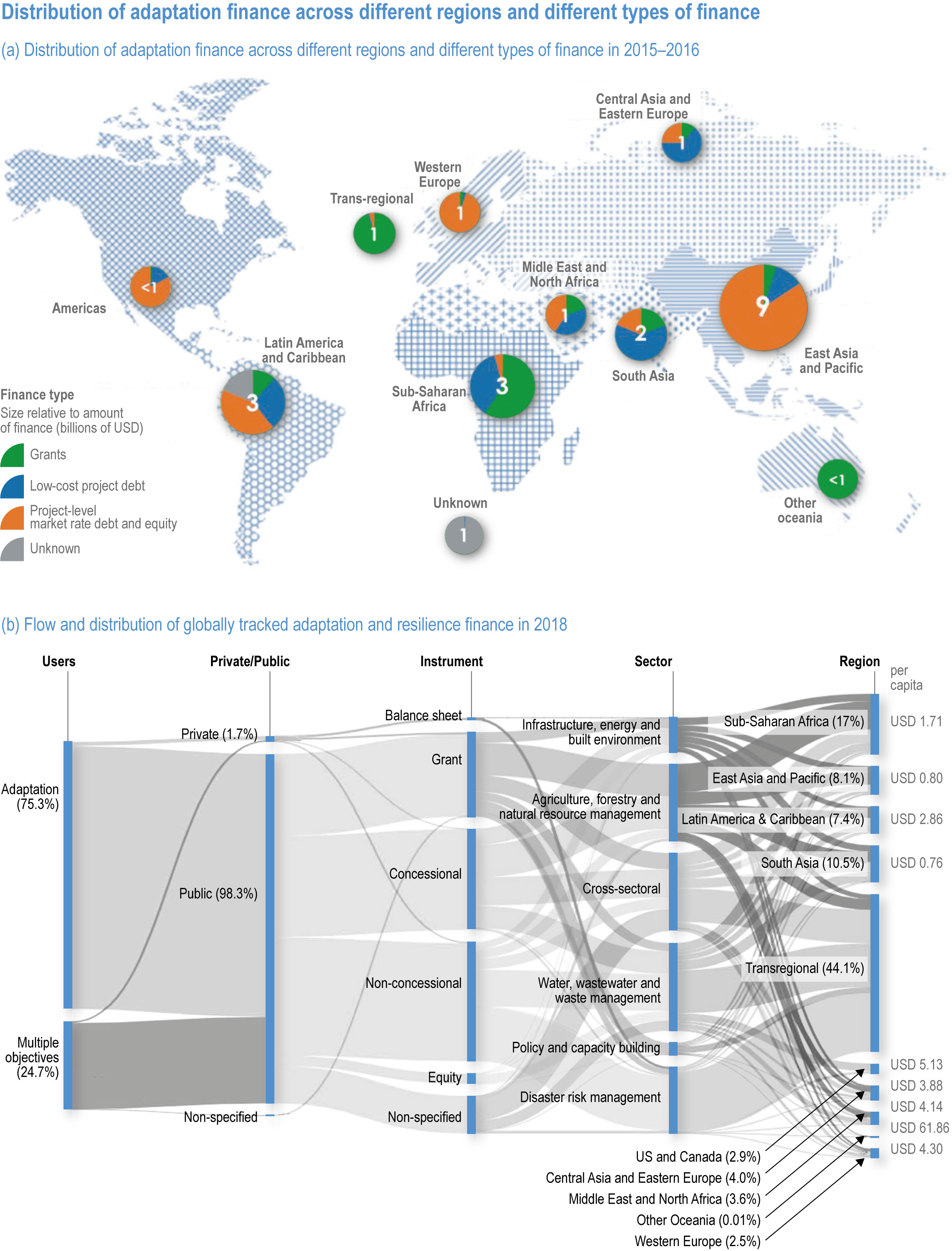 Figure AI.56 | Distribution of adaptation finance across different regions and different types of finance.
